REVIEW 4 major objections 5 minor 40 references
Identification and Computation of Slow Manifolds Using the Isostable Coordinate System
T0 review · 4 major / 5 minor · reviewed 2026-08-06 · deepseek-v4-flash
Pith's one-line read This paper claims that slow manifolds of stable fixed-point systems can be computed backward in time with isostable coordinates, well beyond the linear regime.
desk verdict Genuinely useful isostable-based computation of slow manifolds, but the predictor-corrector's key approximation is not valid in the nonlinear regime and needs serious revision. read the letter →
The pith
A machine-rendered reading of the paper's core claim, the machinery that carries it, and where it could break.
The reading
What carries the argument
The central objects are the principal isostable coordinates $\psi_1,\ldots,\psi_N$\u2014level-set coordinates of the slowest Koopman eigenfunctions, ordered so that each obeys $\dot{\psi}_k=\lambda_k\psi_k$\u2014and their spatial gradients $I_k=\partial\psi_k/\partial x$. The slow manifold is defined as the zero level set of the fast coordinates, $W^s=\{x:\psi_k(x)=0,\ k>\beta\}$. The argument runs through equation (19), an ODE whose right-hand side is the inverse of the matrix of gradients $I_k$ applied to the vector $(-\lambda_1\psi_1,\ldots,-\lambda_\beta\psi_\beta,0,\ldots,0)$; this integrates trajectories exactly along $W^s$ in backward time. Because the slow gradients can be integrated reliably through (20), the only missing ingredient is the span of the fast gradients, supplied either by the asymptotic expansion (35) for $g_1,\ldots,g_\beta$ or by the predictor-corrector projection (42) combined with correction step (46).
What would settle it
Take a system whose slow manifold is known exactly, such as the planar model $\dot{x}_1=-0.05x_1$, $\dot{x}_2=-(x_2-x_1^4+2x_1^2)$, whose slow manifold is the nullcline $x_2=x_1^4-2x_1^2$. Integrate the predictor-corrector scheme (19), (20), (42), (46) backwards far enough into the nonlinear regime and compare the resulting trajectory to the exact curve: if the computed trajectory departs from the known curve before the stated integration range is reached, the projection assumption (42) has failed, and the central claim is refuted for that regime.
Extended reading notes
Core claim
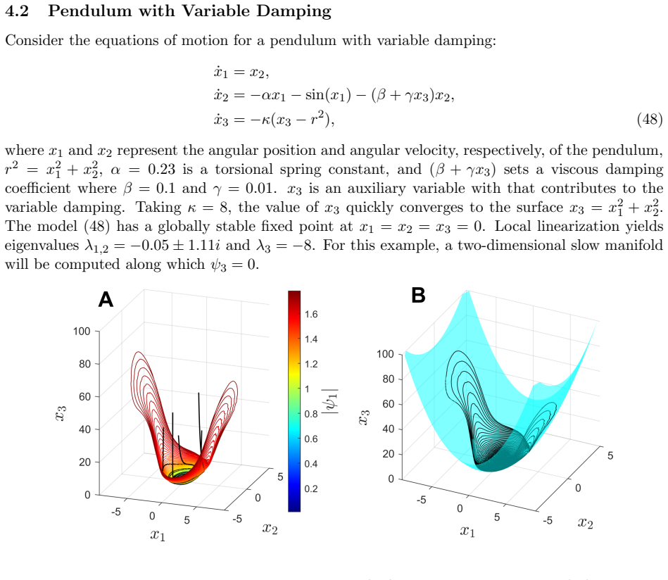
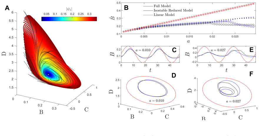
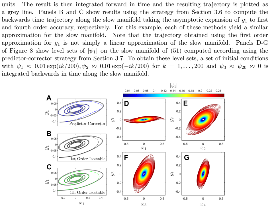
The central claim is that trajectories lying on the slow manifold $W^s = \{x \mid \psi_k(x)=0 \text{ for } k>\beta\}$ can be propagated backward in time from a small neighborhood of the fixed point into the strongly nonlinear region by integrating equation (19), which expresses $dx/d\tilde{t}$ using the gradients $I_k$ of the slow isostable coordinates and zeros out the fast coordinates. The slow gradients $I_1,\ldots,I_\beta$ are computable accurately because adjoint equation (20) suppresses numerical errors over the integration window, while the fast gradient directions are never integrated directly: they are replaced by the span of $g_1,\ldots,g_\beta$, obtained either from a Taylor expansion of the state in isostable coordinates or from the predictor-corrector approximation $g_j(t_1) \approx \sum_{k=1}^\beta (1/(\hat{\lambda}_k \exp(-\lambda_j(t_2-t_1)))) \hat{v}_k \hat{w}_k^T v_j$, which projects onto the slow linear eigenspace. The paper demonstrates on a planar example, a damped pendulum, the Goodwin circadian model, and a ten-oscillator network that the computed surface is invariant under forward flow and yields accurate reduced-order forced models, including reproducing a period-doubling bifurcation that a linearized model misses.
Load-bearing premise
The load-bearing assumption is that, well away from the fixed point, each fast-direction vector stays close enough to the linear slow eigenspace that it can be replaced by its projection; the paper itself notes there is no obvious metric for how far into the nonlinear regime this remains true.
Editorial extensions
If this is right
- If the methods hold, a slow manifold defined by $\psi_k=0$ for $k>\beta$ can be traced from the fixed point into the nonlinear regime, giving a concrete geometric object for model reduction rather than a local linear approximation.
- The one- or two-dimensional isostable reduced models built from the computed manifold reproduce nonlinear forced responses, such as the period-doubling bifurcation of the Goodwin oscillator, that local linearization misses.
- The predictor-corrector strategy only needs local Jacobian evaluations along a trajectory, so it scales to higher-dimensional systems where the asymptotic expansion becomes computationally prohibitive, as demonstrated on a 20-dimensional oscillator network.
- Because forward trajectories converge exponentially fast to the slow manifold, moderate errors in the computed manifold still give useful reduced-order models.
Reading between the lines
- Beyond the paper itself, one could map where the projection assumption (42) breaks down by computing the residual $r_j(t_1)$ along the same trajectory, giving a practical validity horizon for the manifold that could be compared across systems with different spectral gaps.
- Beyond the paper itself, a data-driven variant could estimate $I_1,\ldots,I_\beta$ and the span of $g_1,\ldots,g_\beta$ from short forward simulations, extending the approach to systems whose governing equations are unknown.
- Beyond the paper itself, the correction-step subspace may select one branch of the slow manifold when resonance or near-resonance among eigenvalues makes the expansion (33) non-unique, so uniqueness questions could be studied by varying that projection.
Editorial analysis
A structured set of objections, weighed in public.
Referee Report
Summary. This paper defines the slow manifold of a stable fixed point as the set where the fast principal isostable coordinates vanish, W^s = {x | ψ_k(x)=0 for k>β}, and proposes two computational strategies for following this manifold backwards in time from the fixed point into the nonlinear regime. The first strategy (§3.6) uses an asymptotic expansion of the dual vectors g_j in powers of the isostable coordinates; the second (§3.7) is a predictor-corrector method that approximates g_j by its projection onto the slow eigenspace V_β (Eq. (42)). The backward-time evolution equation (19) is exact given the gradients I_k, and the paper derives evolution equations for I_k and g_k along trajectories. The methods are applied to a planar model, a damped pendulum, the Goodwin oscillator, and a population of coupled planar oscillators, and reduced-order models are constructed that reproduce forced responses and a period-doubling bifurcation missed by linearization.
Significance. The idea of defining slow manifolds through principal isostable coordinates is attractive, and the exact formulation in Eq. (19) is a useful contribution that connects Koopman/isostable theory with geometric slow-manifold reduction. The numerical examples span nontrivial systems, and the reduced-order models show behavior, such as a period-doubling bifurcation and frequency-dependent resonance, that a local linearization misses. However, the central approximation (42) of the predictor-corrector method is an ansatz whose validity the paper itself, in Section 5, says cannot be checked explicitly; moreover, Section 4.1 provides a direct instance where the residual assumption behind (42) fails badly. The advertised claim of accurate backward propagation along W^s is therefore not established, and the numerical successes appear to rely on the forward contraction property rather than on accurate computation of the slow manifold. The paper would be substantially strengthened by reframing what the predictor-corrector algorithm actually computes and by supplying quantitative error measures.
major comments (4)
- [3.7.1, Eq. (42)] The approximation g_j(t1) ≈ ∑_{k=1}^β (1/(\hat{λ}_k exp(-λ_j(t2-t1)))) \hat{v}_k \hat{w}_k^T v_j is load-bearing for the predictor-corrector strategy, but the residual condition ||r_j(t1)||=O(ε) is asserted rather than derived. From (39), r_j(t1) contains the terms (1/(\hat{λ}_k exp(-λ_j(t2-t1)))) \hat{v}_k \hat{w}_k^T(v_j+O(ε)) for k=β+1,...,N. Even when \hat{w}_k^T v_j=0 by biorthogonality, the O(ε) correction at t2 generally has a fast component, and that component is amplified by the reciprocal of \hat{λ}_k exp(-λ_j(t2-t1)), which is exponentially large for k>β. Thus (42) tacitly imposes an additional spectral/nonnormality condition on the O(ε) correction. Section 5 concedes that there is no obvious metric to check this condition, so the central approximation is unverified.
- [4.1, Eq. (47)] For β=1, the planar system (47) has exact slow manifold x2=(5/4)x1^4-(20/9)x1^2 and hence g1=(1,h'(x1))^T with h'=5x1^3-(40/9)x1. The predictor-corrector integration starts near x1=0.001 and, after 150 time units of backward integration, reaches x1≈0.001 exp(0.05·150)=1.8. At x1=1.8, ||r_1||_2=|h'(1.8)|≈21.2, which is not O(ε) for ε=0.001. Equation (42) is therefore violated precisely in the nonlinear regime that the method claims to enter. The favorable result in Figure 3 appears to be produced by the correction step (46) followed by exponential contraction in forward time, not by accurate backward propagation on W^s. The manuscript should either demonstrate backward propagation with quantitative error measures or redefine what the algorithm actually computes.
- [3.4, Eq. (27)] The error analysis for the computation of I_1,...,I_β is heuristic. Equation (27) bounds the error under the assumptions that per-step solver errors are O(ε), that \bar{s}_k||I_k||<O(1/ε), and that the relevant exponential factors remain O(1). The second assumption is state-dependent and is not verified along the computed trajectories, and the analysis does not account for the fact that the trajectory itself is approximate when (19) is integrated. Since (19) requires I_1,...,I_β, this gap is load-bearing. A numerical estimate of the error in I_j along the manifolds of Section 4 would help.
- [4, Figures 3-9] The numerical validation is qualitative throughout. For the planar example, the exact slow manifold is known and the errors of both methods can be tabulated as functions of ψ_1 and of the expansion order, but no error norms are reported. For the pendulum, Goodwin, and coupled-oscillator examples, agreement is assessed visually by forward integration, and the period-doubling bifurcation in Section 4.3 is located at a=0.020 versus the full model's a=0.023 without uncertainty quantification. Given that the checkable hypotheses behind (42) are admitted in Section 5 to be unverifiable, quantitative error measures are needed to support the paper's accuracy claims.
minor comments (5)
- [Abstract] The phrase 'in terms a linear' should read 'in terms of a linear'.
- [Eq. (14)] In the linear solution formula, the sum is over j but the exponential uses λ_k; it should be exp(λ_j t).
- [Eq. (34)] The third-order term in the expansion should involve h_{ijk}, not h_{jk}.
- [4.3, Figure 7 text] The sentence referring to 'initial conditions evolving under the flow of (48)' should refer to the Goodwin model (17), not the pendulum (48).
- [3.7.3, Eq. (46)] The set {\hat{v}_{β+1},...,\hat{v}_{β+N}} should be {\hat{v}_{β+1},...,\hat{v}_N}.
Circularity Check
No significant circularity: the backward-time manifold computation is derived in-line and benchmarked against full-model forward simulations.
full rationale
The claimed derivation chain is self-contained rather than circular. The central backward evolution rule (19) follows directly from the defining isostable dynamics (5) and the chain rule, not from the slow manifold being computed, and the companion gradient equation (6) is proved in the text. The asymptotic-expansion route of Section 3.6 computes g_1,...,g_beta by equating the time derivative of the expansion (33) with (32), with coefficients generated by the recursions in Appendix B; this is a local Taylor-type construction, not an input fitted to the output manifold. The predictor-corrector route of Section 3.7 is an explicitly stated approximation: Eq. (42) is derived under the paper's declared assumptions that r_j(t_1) has O(epsilon) norm and that the relevant minimum singular value is O(1), and Section 5 openly states that 'there is no obvious metric to gauge how far these conditions extend into the nonlinear regime.' The validations compare the computed manifold against forward simulations of the original full-order models, nullclines, and full-model reduced-order responses, which are external benchmarks rather than re-statements of the computational assumptions. Self-citations to earlier isostable-coordinate work supply background and computational technique, but the load-bearing identities are either re-derived in the manuscript or supported by independent existence results such as Kvalheim and Revzen. A possible quantitative failure of the O(epsilon) residual condition in a particular example would be a numerical-validity limitation, not a circular step, since the paper does not use the target manifold to enforce the condition. Overall, the predictions are not equivalent to the inputs by construction.
Assumptions & free parameters
free parameters (3)
- Δt (predictor-corrector step) =
0.25 to 0.5 in examples
- Asymptotic expansion order for g_k =
1st to 8th order depending on example
- Initial condition amplitude ε for ψ coordinates =
0.001 to 0.1
assumptions (5)
- domain assumption Principal isostable coordinates ψ_1,...,ψ_N exist and are smooth in the basin of attraction of the fixed point.
- domain assumption The Jacobian J at the fixed point is diagonalizable and the eigenvalues are nonresonant.
- domain assumption The matrix of isostable gradients [I_1^T;...;I_N^T] is invertible along the slow manifold.
- ad hoc to paper The residual r_j(t_1) from Eq. (41) is O(ε) along the backward trajectory.
- ad hoc to paper The minimum singular value of [\hat{v}_{β+1} ... \hat{v}_N] is O(1).
Cite this review
Pith. "Pith review of Identification and Computation of Slow Manifolds Using the Isostable Coordinate System." pith.science (2026). https://pith.science/paper/ZAIC4E4C
@misc{pith2026250713997,
  author       = {Pith},
  title        = {Pith review of: Identification and Computation of Slow Manifolds Using the Isostable Coordinate System},
  year         = {2026},
  howpublished = {\url{https://pith.science/paper/ZAIC4E4C}},
  note         = {Machine review of arXiv:2507.13997}
}
read the original abstract
Koopman analysis can be used to understand the dynamics of a nonlinear dynamical system in terms a linear, but generally infinite dimensional operator. The isostable coordinate system focuses on the slowest decaying principal Koopman eigenmodes. This work leverages the isostable coordinate framework in the identification of slow manifolds for dynamical systems with fixed point attractors, defined as surfaces for which the fastest decaying isostable coordinates are zero. Numerical challenges associated with separation between fast and slow timescales necessitate the development of new computational approaches to identify these slow manifolds. Two such strategies are developed which approximate backward-time solutions on the slow manifold starting near the fixed point and extending far beyond the linear regime. Application to a variety of examples illustrates the utility of these methods and their potential use for model order reduction purposes.
Figures


Figures from the paper (6 more)



Reference graph
Works this paper leans on
-
[1]
Ahmed, A
T. Ahmed, A. Sadovnik, and D. Wilson. Data-driven inference of low-order isostable- coordinate-based dynamical models using neural networks. Nonlinear Dynamics, 111(3):2501– 2519, 2023
2023
-
[2]
U. M. Ascher and L. R. Petzold. Computer methods for ordinary differential equations and differential-algebraic equations, volume 61. SIAM, Philadelphia, 1998
work page 1998
-
[3]
Benner, S
P. Benner, S. Gugercin, and K. Willcox. A survey of projection-based model reduction methods for parametric dynamical systems. SIAM Review, 57(4):483–531, 2015
2015
-
[4]
G. Berkooz, P. Holmes, and J. L. Lumley. The proper orthogonal decomposition in the analysis of turbulent flows. Annual Review of Fluid Mechanics , 25(1):539–575, 1993
work page 1993
-
[5]
S. L. Brunton, B. W. Brunton, J. L. Proctor, and J. N. Kutz. Koopman invariant subspaces and finite linear representations of nonlinear dynamical systems for control. PloS One , 11(2), 2016. 23
work page 2016
-
[6]
M. Budiˇ si´ c, R. Mohr, and I. Mezi´ c. Applied Koopmanism.Chaos: An Interdisciplinary Journal of Nonlinear Science , 22(4):047510, 2012
work page 2012
-
[7]
M. Cenedese, J. Ax ˚ as, B. B¨ auerlein, K. Avila, and G. Haller. Data-driven modeling and prediction of non-linearizable dynamics via spectral submanifolds. Nature Communications, 13(1):872, 2022
work page 2022
-
[8]
Farjami, V
S. Farjami, V. Kirk, and H. M. Osinga. Computing the stable manifold of a saddle slow manifold. SIAM Journal on Applied Dynamical Systems , 17(1):350–379, 2018
2018
Show all 40 references
-
[9]
Fenichel
N. Fenichel. Geometric singular perturbation theory for ordinary differential equations.Journal of differential equations , 31(1):53–98, 1979
1979
-
[10]
Gonze, S
D. Gonze, S. Bernard, C. Waltermann, A. Kramer, and H. Herzel. Spontaneous synchronization of coupled circadian oscillators. Biophysical Journal, 89(1):120–129, 2005
2005
-
[11]
Guckenheimer and C
J. Guckenheimer and C. Kuehn. Computing slow manifolds of saddle type. SIAM Journal on Applied Dynamical Systems , 8(3):854–879, 2009
2009
-
[12]
Gugercin and A
S. Gugercin and A. C. Antoulas. A survey of model reduction by balanced truncation and some new results. International Journal of Control , 77(8):748–766, 2004
2004
-
[13]
Haller and S
G. Haller and S. Ponsioen. Nonlinear normal modes and spectral submanifolds: existence, uniqueness and use in model reduction. Nonlinear Dynamics, 86:1493–1534, 2016
2016
-
[14]
Holmes, J
P. Holmes, J. L. Lumley, G. Berkooz, and C. W. Rowley. Turbulence, coherent structures, dynamical systems and symmetry . Cambridge University Press, New York, 1996
1996
-
[15]
Kaiser, J
E. Kaiser, J. N. Kutz, and S. Brunton. Data-driven discovery of Koopman eigenfunctions for control. Machine Learning: Science and Technology , 2021
2021
-
[16]
T. J. Kaper. Systems theory for singular perturbation problems. In Analyzing multiscale phenomena using singular perturbation methods , pages 85–131. AMS, 1999
1999
-
[17]
J. N. Kutz, S. L. Brunton, B. W. Brunton, and J. L. Proctor. Dynamic mode decomposition: data-driven modeling of complex systems . Society for Industrial and Applied Mathematics, Philadelphia, PA, 2016
2016
-
[18]
M. D. Kvalheim and S. Revzen. Existence and uniqueness of global Koopman eigenfunctions for stable fixed points and periodic orbits. Physica D: Nonlinear Phenomena , page 132959, 2021
2021
-
[19]
Lusch, J
B. Lusch, J. N. Kutz, and S. L. Brunton. Deep learning for universal linear embeddings of nonlinear dynamics. Nature Communications, 9(1):1–10, 2018
2018
-
[20]
Mauroy and I
A. Mauroy and I. Mezi´ c. Global stability analysis using the eigenfunctions of the Koopman operator. IEEE Transactions on Automatic Control , 61(11):3356–3369, 2016
2016
-
[21]
Mauroy, I
A. Mauroy, I. Mezi´ c, and J. Moehlis. Isostables, isochrons, and Koopman spectrum for the action–angle representation of stable fixed point dynamics. Physica D: Nonlinear Phenomena , 261:19–30, 2013
2013
-
[22]
I. Mezi´ c. Analysis of fluid flows via spectral properties of the Koopman operator. Annual Review of Fluid Mechanics , 45:357–378, 2013. 24
2013
-
[23]
I. Mezi´ c. Spectrum of the Koopman operator, spectral expansions in functional spaces, and state-space geometry. Journal of Nonlinear Science , pages 1–55, 2019
2019
-
[24]
B. Moore. Principal component analysis in linear systems: controllability, observability, and model reduction. IEEE Transactions on Automatic Control , 26(1):17–32, 1981
1981
-
[25]
Ponsioen, S
S. Ponsioen, S. Jain, and G. Haller. Model reduction to spectral submanifolds and forced- response calculation in high-dimensional mechanical systems. Journal of Sound and Vibration , 488:115640, 2020
2020
-
[26]
P. J. Schmid. Dynamic mode decomposition of numerical and experimental data. Journal of Fluid Mechanics, 656:5–28, 2010
2010
-
[27]
Sootla and A
A. Sootla and A. Mauroy. Geometric properties of isostables and basins of attraction of monotone systems. IEEE Transactions on Automatic Control , 62(12):6183–6194, 2017
2017
-
[28]
D. C. Sorensen and A. C. Antoulas. The Sylvester equation and approximate balanced reduc- tion. Linear Algebra and its Applications , 351:671–700, 2002
2002
-
[29]
Towne, O
A. Towne, O. T. Schmidt, and T. Colonius. Spectral proper orthogonal decomposition and its relationship to dynamic mode decomposition and resolvent analysis. Journal of Fluid Mechanics, 847:821–867, 2018
2018
-
[30]
S. Wiggins. Introduction to applied nonlinear dynamical systems and chaos, volume 2. Springer, 2003
2003
-
[31]
M. O. Williams, I. G. Kevrekidis, and C. W. Rowley. A data–driven approximation of the koopman operator: Extending dynamic mode decomposition. Journal of Nonlinear Science , 25(6):1307–1346, 2015
2015
-
[32]
D. Wilson. A data-driven phase and isostable reduced modeling framework for oscillatory dynamical systems. Chaos: An Interdisciplinary Journal of Nonlinear Science , 30(1):013121, 2020
2020
-
[33]
D. Wilson. Phase-amplitude reduction far beyond the weakly perturbed paradigm. Physical Review E, 101(2):022220, 2020
2020
-
[34]
D. Wilson. Analysis of input-induced oscillations using the isostable coordinate framework. Chaos: An Interdisciplinary Journal of Nonlinear Science , 31(2):023131, 2021
2021
-
[35]
D. Wilson. Data-driven inference of high-accuracy isostable-based dynamical models in response to external inputs. Chaos: An Interdisciplinary Journal of Nonlinear Science , 31(6):063137, 2021
2021
-
[36]
Wilson and S
D. Wilson and S. Djouadi. Isostable reduction and boundary feedback control for nonlinear convective flow. In Proceedings of the 58th IEEE Conference on Decision and Control , 2019
2019
-
[37]
Wilson and B
D. Wilson and B. Ermentrout. Greater accuracy and broadened applicability of phase reduction using isostable coordinates. Journal of Mathematical Biology , 76(1-2):37–66, 2018
2018
-
[38]
Wilson and J
D. Wilson and J. Moehlis. Extending phase reduction to excitable media: Theory and appli- cations. SIAM Review, 57(2):201–222, 2015. 25
2015
-
[39]
Wilson and J
D. Wilson and J. Moehlis. Isostable reduction of periodic orbits. Physical Review E , 94(5):052213, 2016
2016
-
[40]
Wilson and J
D. Wilson and J. Moehlis. Isostable reduction with applications to time-dependent partial differential equations. Physical Review E , 94(1):012211, 2016. 26
2016
Reviewed August 6, 2026 · model on record in the stance chip above.
Discussion (0). Continue with ORCID to comment.