REVIEW 3 major objections 6 minor 38 references
A Stability-Driven Framework for Long-Term Hourly Electricity Demand Forecasting
T0 review · 3 major / 6 minor · reviewed 2026-08-06 · deepseek-v4-flash
Pith's one-line read Hourly electricity demand can be forecast five years ahead with under seven percent error by combining a GDP regression with the observation that the hourly shape of demand is stable across years.
desk verdict A sensible and reproducible long-term hourly load forecasting method, but the headline 'six-year-ahead' accuracy is actually a four-year-ahead result and the paper needs to correct that and several statistical issues. read the letter →
The pith
A machine-rendered reading of the paper's core claim, the machinery that carries it, and where it could break.
The reading
What carries the argument
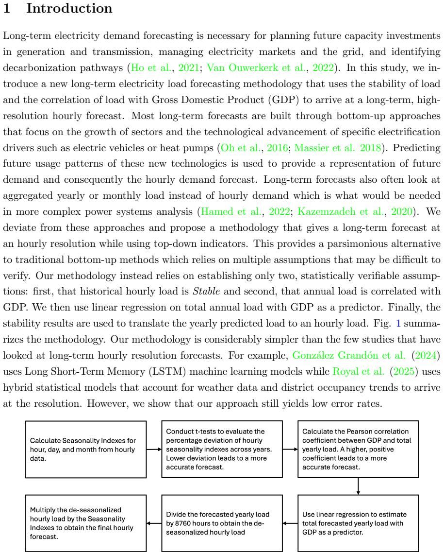
The load-bearing object is the seasonality index (SI), a multiplicative factor measuring how much demand in a given month, day of the week, or hour deviates from the yearly average, computed in three nested levels: $\mathrm{SI}^1_{y,m}$ for months, $\mathrm{SI}^2_{y,m,d}$ for days of the week, and $\mathrm{SI}^3_{y,m,d,h}$ for hours. Stability is defined operationally: for every hour and day, a series of two-sample one-tailed t-tests between all pairwise years finds the smallest $\epsilon$ such that the null hypothesis of a difference at least $\epsilon$ is rejected, yielding the largest average shift of each index. The forecast then uses a baseline year's indices as a fixed distribution: the GDP-regressed yearly total is deseasonalized to an average hour, and that average is multiplied by the stored $\mathrm{SI}^1$, $\mathrm{SI}^2$, and $\mathrm{SI}^3$ values to rebuild the hourly curve.
What would settle it
Recompute the hourly seasonality indices on data from a later window, for example 2023-2025 for Singapore, and compare them with the 2004-2022 means: if the average absolute deviation exceeds the measured 4.24 percent, or the per-hour values exceed the epsilons in the paper's Table 2, the stability premise fails and hourly errors should exceed the reported MAPE bound. A weaker but still decisive test is to run the full procedure on a country with rapid rooftop-solar or EV growth and check whether hourly MAPE over a four-year horizon grows while annual MAPE stays small.
Extended reading notes
Core claim
The central discovery the paper argues for is that hourly load shapes are stable enough over multi-year horizons to serve directly as a forecasting device. Multiplicatively decomposing Singapore's half-hourly demand into monthly, day-of-week, and hour-of-day seasonality indices, the paper finds that the largest pairwise year-to-year differences in the hourly indices average just 4.24 percent of the mean index (4.65 percent on weekdays, 3.21 percent on weekends), as verified through paired t-tests. Because annual electricity consumption correlates with GDP (Pearson coefficient 0.9947 for Singapore), a simple linear regression on GDP supplies the yearly total, and the stable indices from the baseline year convert that total into an hourly curve. The reported errors, a maximum 6.87 percent MAPE across six forecast years for Singapore and 6.81 and 5.64 percent for Belgium and Bulgaria, are the paper's evidence that the stability-plus-GDP recipe carries the entire forecasting burden.
Load-bearing premise
The forecast inherits the shape of the daily demand curve from a baseline year, so if the relative hourly pattern shifts materially over the four-to-five-year horizon, through new technology, changed working habits, or a different generation mix, the hourly forecast remains wrong even when the annual total is right.
Editorial extensions
If this is right
- A grid planner can produce a defensible hourly load curve for a five-year horizon using only historical load data and GDP, without modeling electrification drivers such as EV or heat-pump uptake.
- Hourly error stays below 7 percent even when the yearly-total forecast misses by up to 6.12 percent, so in these cases the seasonality-index distribution is not the dominant error source.
- The stability diagnosis transfers across economies: an OECD country (Belgium, 8.41 percent SI deviation) and a non-OECD country (Bulgaria, 13.24 percent) both yield two-year-ahead hourly MAPEs under 7 percent.
- Constancy of the seasonality indices lets a Holt-Winters exponential smoothing model fix its seasonal components and optimize only two smoothing constants, matching or beating machine-learning benchmarks in most years.
- Any improved yearly-total forecast can be plugged into the same stability machinery to obtain an hourly curve, so the seasonality-index framework is separable from the GDP regression.
Reading between the lines
- If hourly shape stability is the real engine, accuracy should degrade precisely where the shape changes, through large rooftop-solar fleets, EV charging ramps, or work-from-home shifts, even when annual GDP correlation holds; a direct test would recompute the seasonality indices for 2023-2025 and compare them with the 2004-2022 baseline.
- The paper's worst errors occur in the COVID-recovery years, which suggests the method inherits whatever error the GDP regression makes on the yearly total, so macroeconomic shocks dominate the error budget rather than the stability assumption.
- The paper itself flags that GDP decoupling in OECD economies and rapid electrification in non-OECD economies can weaken the predictor, so the sensible deployment is as a baseline curve corrected for known structural changes rather than a blind extrapolation.
- The epsilon-search t-test effectively measures the largest average pairwise drift of each index; a complementary check would compare the seasonality-index distribution from a training window directly against a hold-out window, which the baseline-year design already makes possible.
Editorial analysis
A structured set of objections, weighed in public.
Referee Report
Summary. The paper proposes a parsimonious, top-down framework for long-term hourly electricity demand forecasting. Seasonality indices for month, day of week, and hour are computed from historical load data; pairwise t-tests with an epsilon-adjustment are used to argue that these indices are stable over time. Annual load is regressed on GDP via simple linear regression, and the resulting annual forecast is distributed to individual hours using the baseline year's seasonality indices. The method is applied to Singapore (2004-2022), Belgium, and Bulgaria, with claimed maximum MAPEs of 6.87%, 6.81%, and 5.64%. The stability indices are also plugged into an exponential smoothing model for short-term forecasting and compared with several machine-learning benchmarks.
Significance. If the results hold, the paper offers a notable counterpoint to complex bottom-up and machine-learning approaches: a transparent, low-parameter method for long-term hourly load forecasting, validated in three countries with different economic characteristics. The use of publicly available data, the explicit focus on statistical verification of stability, and the cross-country extension are strengths. However, the headline claim is weakened by an inconsistent and apparently overstated forecast-horizon label, and the stability test is presented without the statistical detail needed to assess its validity. The short-term extension also contains a look-ahead bias. The core idea is plausible and potentially useful, but the evidence as presented is not yet fully convincing.
major comments (3)
- [Abstract and Section 3.1] The forecast horizon is mislabeled in a way that affects the central claim. Section 3.1 states that the models predict 'total yearly load in baseline year + 4', and Table 6 lists forecast years 2017-2022 with baseline years 2013-2018, which is a four-year gap in each case. Yet the abstract claims 'six-year-ahead forecasts' and Section 3 states '5-year ahead forecasts'. Figure 5 further uses baseline year 2014 for a 2019 sample week, a five-year gap. The stated maximum MAPE of 6.87% is therefore for four-year-ahead forecasts, not six-year-ahead. Because the horizon is an intrinsic part of the contribution's claimed difficulty, this mislabeling must be corrected in the abstract, Section 3, the conclusion, and Figure 5, or the experiments must actually be run at the stated horizons.
- [Section 2.2.4] The t-test procedure for stability is not fully specified and, as described, does not appear to be a standard statistical test. The text does not report the significance level (alpha) used for the two one-tailed t-tests. The procedure increments epsilon by 0.001 until both null hypotheses are rejected; the final epsilon is then interpreted as the 'maximum difference'. With 19 years, there are 171 pairwise year comparisons for each of 168 hour-by-day combinations, so tens of thousands of tests are performed, yet no multiple-testing correction is mentioned. The reported quantities are therefore data-dependent, and their statistical meaning is unclear. Please specify the significance level, describe how multiple testing is handled (the error rate is otherwise uncontrollable), or present the analysis explicitly as a descriptive stability measure rather than as a formal hypothesis test.
- [Section 5 and Table 7] The short-term exponential smoothing extension uses the full-sample seasonality indices mu_{d,h} from 2004-2022 (Section 5 states 'we make use of the overall seasonality indices ... from (9)') and then evaluates the model on 2018-2022. This means the seasonality components are estimated on data that include the evaluation period, a look-ahead bias. The comparison with machine-learning methods that are fit only on the training period is therefore favorable to the proposed ES model. The seasonality indices should be estimated recursively using only data up to each forecast origin, or the limitation should be explicitly acknowledged and the comparison revisited.
minor comments (6)
- [Abstract] The abstract refers to both 'five-year-ahead total yearly forecasts' and 'six-year-ahead forecasts' for the same experiments; these labels are inconsistent and need to be reconciled with the actual horizons.
- [Section 2.1] The half-hourly to hourly transformation is described with care, but the statement that summing two half-hourly MW values 'is equivalent to 5700MWh' could be clearer: the sum in MW equals the energy in MWh only for a one-hour integration period; consider a more explicit unit conversion.
- [Tables 4 and 5] All p-values are reported as '0.00'; they should be reported as '< 0.001' or similar to reflect that they are rounded.
- [Table 6] The column headers 'Percentage Error (Total Year)' and 'Percentage Error (Hourly)' do not indicate whether these are absolute percentage errors; MAPE implies absolute values elsewhere, so consider renaming for consistency.
- [Section 4] The statement that the model was 'trained using the 2006-2017 dataset' is imprecise: the only fitted component is the linear regression on GDP, and the data are used for both regression and seasonality indices; please specify which parts are estimated on which periods.
- [Section 2.2.4] The description of the right-tailed test contains a typo: the null hypothesis should likely be 'mu_y - mu_y' <= epsilon' rather than 'mu_y - mu_y' <= -epsilon', as written the two tests appear asymmetric.
Circularity Check
One secondary 'prediction' (the short-term ES model) is partly in-sample because its seasonality indices are averaged over the target years, but the central long-term GDP-based hourly forecast is self-contained.
-
fitted input called prediction
[Section 5, Eq. (9) and Table 7]
"We then make use of the overall seasonality indices for month, day, and year µd,h from (9) as proxies for the seasonality index calculations in the ES model above. That is, we assume that the S^i_t are constant. ... (9): µd,h = P2022 y=2004 P12 m=1 SI3 y,m,d,h / ((2022−2004+1)(12))."
µd,h is the average of the hourly seasonality indices over 2004–2022, which includes the forecast years 2018–2022 evaluated in Table 7. These full-sample indices are then fixed as the S^i_t terms in the Holt-Winters ES model and used to produce the day-ahead 'forecasts' reported in Table 7. The seasonal shape of each target year is therefore constructed, by Eq. (9), from the actual data of that same target year, so those MAPEs are not out-of-sample predictions of hourly shape but in-sample fits. This is a look-ahead, fitted-input-called-prediction reduction, though it is confined to the short-term extension and does not enter the long-term baseline-year forecasting chain.
full rationale
The central long-term forecasting claim is not circular. The total yearly load is predicted from IMF GDP forecasts via a regression fit only through the baseline year, and the hourly distribution is obtained by multiplying that yearly total by SI indices from the baseline year (y−4), not from the target year. The stability analysis in Section 2 is an independent statistical verification (t-tests on historical SIs) rather than an assumption imported from the result. No load-bearing self-citation chain is present. The principal circularity concern is the short-term ES extension: Eq. (9) defines µd,h over 2004–2022, and Section 5 sets the ES seasonality terms equal to these full-sample values before reporting MAPEs for 2018–2022, so those particular hourly 'forecasts' are partly in-sample by construction. Because the headline long-term hourly forecast (the 6.87% max MAPE claim) does not reduce to its inputs and the ES leakage is a secondary extension, the overall circularity score is 4 rather than 6 or higher. The inconsistent 'five- vs six-year ahead' horizon labels are a correctness/consistency issue, not a circularity issue.
Assumptions & free parameters
free parameters (2)
- Linear regression intercept and slope (per baseline year) =
Intercepts 58.8M-61.1M; slopes 115,679-129,589 (Tables 4-5)
- Exponential smoothing constants alpha and beta =
alpha = 0.19, beta = 0.88
assumptions (4)
- domain assumption Seasonality indices are stable over multi-year horizons
- domain assumption Annual electricity load is linearly related to GDP
- domain assumption GDP forecasts from IMF WEO are accurate enough for forecasting
- ad hoc to paper The t-test procedure provides a valid measure of stability
Cite this review
Pith. "Pith review of A Stability-Driven Framework for Long-Term Hourly Electricity Demand Forecasting." pith.science (2026). https://pith.science/paper/5KP4OIZ4
@misc{pith2026250715001,
  author       = {Pith},
  title        = {Pith review of: A Stability-Driven Framework for Long-Term Hourly Electricity Demand Forecasting},
  year         = {2026},
  howpublished = {\url{https://pith.science/paper/5KP4OIZ4}},
  note         = {Machine review of arXiv:2507.15001}
}
read the original abstract
Long-term electricity demand forecasting is essential for grid and operations planning, as well as for the analysis and planning of energy transition strategies. However, accurate long-term load forecasting with high temporal resolution remains challenging, as most existing approaches focus on aggregated forecasts, which require accurate prediction of numerous variables for bottom-up sectoral forecasts. In this study, we propose a parsimonious methodology that employs t-tests to verify load stability and the correlation of load with gross domestic product (GDP) to produce a long-term hourly load forecast. Applying this method to Singapore's electricity demand, analysis of multi-year historical data (2004-2022) reveals that its relative hourly load has remained statistically stable, with an overall percentage deviation of 4.24% across seasonality indices. Utilizing these stability findings, five-year-ahead total yearly forecasts were generated using GDP as a predictor, and hourly loads were forecasted using hourly seasonality index fractions. The maximum Mean Absolute Percentage Error (MAPE) across multiple experiments for six-year-ahead forecasts was 6.87%. The methodology was further applied to Belgium (an OECD country) and Bulgaria (a non-OECD country), yielding MAPE values of 6.81% and 5.64%, respectively. Additionally, stability results were incorporated into a short-term forecasting model based on exponential smoothing, demonstrating comparable or improved accuracy relative to existing machine learning-based methods. These findings indicate that parsimonious approaches can effectively produce long-term, high-resolution forecasts.
Figures


Figures from the paper (7 more)


Reference graph
Works this paper leans on
-
[1]
Bandara, K., Hyndman, R. J., and Bergmeir, C. (2021). MSTL : A Seasonal - Trend Decomposition Algorithm for Time Series with Multiple Seasonal Patterns . http://arxiv.org/abs/2107.13462. [Online; accessed 13-Dec-2023]
arXiv 2021
-
[2]
Bazán Navarro , C. E., Morocho Ruiz , J. D., and Castillo Alvarado , J. F. (2024). Economic growth and electricity consumption: Fresh evidence of panel data for lac. Heliyon , 10(13):e33521
work page 2024
-
[3]
Bouktif, S., Fiaz, A., Ouni, A., and Serhani, M. (2018). Optimal Deep Learning LSTM Model for Electric Load Forecasting using Feature Selection and Genetic Algorithm : Comparison with Machine Learning Approaches . Energies , 11(7):1636
work page 2018
-
[4]
Chuan, L. and Ukil, A. (2015). Modeling and Validation of Electrical Load Profiling in Residential Buildings in Singapore . IEEE Transactions on Power Systems , 30(5):2800--2809
work page 2015
-
[5]
De Felice , M., Alessandri, A., and Catalano, F. (2015). Seasonal climate forecasts for medium-term electricity demand forecasting. Applied Energy , 137:435--444
work page 2015
-
[6]
Deng, J. and Jirutitijaroen, P. (2010). Short-term load forecasting using time series analysis: A case study for Singapore . In 2010 IEEE Conference on Cybernetics and Intelligent Systems , pages 231--236, , Singapore. IEEE
work page 2010
-
[7]
Half-hourly System Demand Data
EMA (2023). Half-hourly System Demand Data . https://www.ema.gov.sg/resources/statistics/half-hourly-system-demand-data. [Online; accessed 01-Jul-2023]
work page 2023
-
[8]
ENTSOE (2023). europe. https://www.entsoe.eu/data/power-stats/. [Online; accessed 01-Mar-2025]
work page 2023
Show all 38 references
-
[9]
González Grandón, T., Schwenzer, J., Steens, T., and Breuing, J. (2024). Electricity demand forecasting with hybrid classical statistical and machine learning algorithms: Case study of Ukraine . Applied Energy , 355:122249
2024
-
[10]
M., Ali, H., and Abdelal, Q
Hamed, M. M., Ali, H., and Abdelal, Q. (2022). Forecasting annual electric power consumption using a random parameters model with heterogeneity in means and variances. Energy , 255:124510
2022
-
[11]
A., Jereb, B., Rosi, B., and Dragan, D
Hammad, M. A., Jereb, B., Rosi, B., and Dragan, D. (2020). Methods and Models for Electric Load Forecasting : A Comprehensive Review . Logistics & Sustainable Transport , 11(1):51--76
2020
-
[12]
Ho, J., Becker, J., Brown, M., Brown, P., Chernyakhovskiy, I., Cohen, S., Cole, W., and et al. (2021). Regional Energy Deployment System ( ReEDS ) Model Documentation : Version 2020. https://www.nrel.gov/docs/fy21osti/78195.pdf
2021
-
[13]
Huang, J., Srinivasan, D., and Zhang, D. (2017). Electricity Demand Forecasting Using HWT Model with Fourfold Seasonality . In 2017 International Conference on Control , Artificial Intelligence , Robotics & Optimization ( ICCAIRO ) , pages 254--258, Prague. IEEE
2017
-
[14]
and Athanasopoulos, G
Hyndman, R. and Athanasopoulos, G. (2018). Forecasting: Principles and Practice . OTexts, Australia, 2nd edition
2018
-
[15]
World Economic Outlook Database
IMF (2023). World Economic Outlook Database . https://www.imf.org/en/Publications/WEO/weo-database/2023/October. [Online; accessed 5-Mar-2024]
2023
-
[16]
Kazemzadeh, M.-R., Amjadian, A., and Amraee, T. (2020). A hybrid data mining driven algorithm for long term electric peak load and energy demand forecasting. Energy , 204:117948
2020
-
[17]
Konica, J. A. (2016). Forecasting Next - Day the Electricity Demand Based On Fuzzy Logic Method Case for Albania . 3(12)
2016
-
[18]
Korstanje, J. (2021). The SARIMAX Model . In Advanced Forecasting with Python : With State -of-the- Art - Models Including LSTMs , Facebook 's Prophet , and Amazon 's DeepAR , pages 125--131. Apress, Berkeley, CA
2021
-
[19]
Loi, T. S. A. and Loo, S. L. (2016). The impact of singapore’s residential electricity conservation efforts and the way forward. insights from the bounds testing approach. Energy Policy , 98:735--743
2016
-
[20]
Loi, T. S. A. and Ng, J. L. (2018). Analysing households’ responsiveness towards socio-economic determinants of residential electricity consumption in singapore. Energy Policy , 112:415--426
2018
-
[21]
Massier, T., Recalde, D., Sellmair, R., Gallet, M., and Hamacher, T. (2018). Electrification of Road Transport in Singapore and its Integration into the Power System . Energy Technology , 6(1):21--32
2018
-
[22]
A., Alghassab, M., Ullah, K., Khan, Z
Mir, A. A., Alghassab, M., Ullah, K., Khan, Z. A., Lu, Y., and Imran, M. (2020). A review of electricity demand forecasting in low and middle income countries: The demand determinants and horizons. Sustainability , 12(15)
2020
-
[23]
Neo, H. Y. R., Wong, N. H., Ignatius, M., and Cao, K. (2023). A hybrid machine learning approach for forecasting residential electricity consumption: A case study in Singapore . Energy & Environment , page 0958305X2311740
2023
-
[24]
K., Teimeh, M., Nyarko-Boateng, O., and Adekoya, A
Nti, I. K., Teimeh, M., Nyarko-Boateng, O., and Adekoya, A. F. (2020). Electricity load forecasting: a systematic review. Journal of Electrical Systems and Information Technology , 7(1):13
2020
-
[25]
J., Ng, K
Oh, S. J., Ng, K. C., Thu, K., Chun, W., and Chua, K. J. E. (2016). Forecasting long-term electricity demand for cooling of Singapore ’s buildings incorporating an innovative air-conditioning technology. Energy and Buildings , 127:183--193
2016
-
[26]
correlation
OWID (2023). correlation. https://nyc3.digitaloceanspaces.com/owid-public/data/energy/owid-energy-data.csv. [Online; accessed 01-Mar-2025]
2023
-
[27]
Pełka, P. (2023). Analysis and forecasting of monthly electricity demand time series using pattern-based statistical methods. Energies , 16(2)
2023
-
[28]
T., Chetangny, P
Prodjinotho, U. T., Chetangny, P. K., Agbomahena, M. B., Zogbochi, V., Medewou, L., Barbier, G., and Chamagne, D. (2024). Long term forecasting of peak demand and annual electricity consumption of the west african power pool interconnected network by 2032. International Journa...
2024
-
[29]
Quan, H., Srinivasan, D., and Khosravi, A. (2014). Short- Term Load and Wind Power Forecasting Using Neural Network - Based Prediction Intervals . IEEE Transactions on Neural Networks and Learning Systems , 25(2):303--315
2014
-
[30]
and Peng, J
Raman, G. and Peng, J. C.-H. (2021). Electricity consumption of singaporean households reveals proactive community response to covid-19 progression. Proceedings of the National Academy of Sciences , 118(34):e2026596118
2021
-
[31]
Royal, E., Bandyopadhyay, S., Newman, A., Huang, Q., and Tabares-Velasco, P. C. (2025). A statistical framework for district energy long-term electric load forecasting. Applied Energy , 384:125445
2025
-
[32]
A., and Shahzad, S
Sharif, A., Jammazi, R., Raza, S. A., and Shahzad, S. J. H. (2017). Electricity and growth nexus dynamics in Singapore : Fresh insights based on wavelet approach. Energy Policy , 110:686--692
2017
-
[33]
Steinbuks, J., de Wit, J., Kochnakyan, A., and Foster, V. (2017). Forecasting electricity demand: An aid for practitioners. Technical Report 2017/73, World Bank, Washington, DC. © World Bank
2017
-
[34]
Taylor, S. J. and Letham, B. (2017a). Forecasting at scale. https://peerj.com/preprints/3190v2. [Online; accessed 13-Dec-2023]
2017
-
[35]
Taylor, S. J. and Letham, B. (2017b). Prophet: forecasting at scale. https://research.facebook.com/blog/2017/2/prophet-forecasting-at-scale/. [Online; accessed 13-Dec-2023]
2017
-
[36]
C., Gardian, H., Kittel, M., Schill, W.-P., Zerrahn, A., Murmann, A., Launer, J., Torralba-Díaz, L., and Bußar, C
Van Ouwerkerk, J., Gils, H. C., Gardian, H., Kittel, M., Schill, W.-P., Zerrahn, A., Murmann, A., Launer, J., Torralba-Díaz, L., and Bußar, C. (2022). Impacts of power sector model features on optimal capacity expansion: A comparative study. Renewable and Sustainable Energy Re...
2022
-
[37]
C., Pedregal, D
Young, P. C., Pedregal, D. J., and Tych, W. (1999). Dynamic harmonic regression. Journal of Forecasting , 18(6):369--394
1999
-
[38]
Zahid, M., Ahmed, F., Javaid, N., Abbasi, R., Zainab Kazmi, H., Javaid, A., Bilal, M., Akbar, M., and Ilahi, M. (2019). Electricity Price and Load Forecasting using Enhanced Convolutional Neural Network and Enhanced Support Vector Regression in Smart Grids . Electronics , 8(2):122
2019
Reviewed August 6, 2026 · model on record in the stance chip above.
Discussion (0). Sign in to comment.