REVIEW 3 major objections 4 minor 59 references
Binary Response Forecasting under a Factor-Augmented Framework
T0 review · 3 major / 4 minor · reviewed 2026-08-06 · deepseek-v4-flash
Pith's one-line read The paper proposes a factor-augmented probit for binary outcomes and claims it beats conventional probit in U.S. recession forecasting, with a central limit theorem enabling inference.
desk verdict A useful binary-response FAR theory with real asymptotics, but the empirical superiority claim needs serious fixing before it should be accepted. read the letter →
The pith
A machine-rendered reading of the paper's core claim, the machinery that carries it, and where it could break.
The reading
What carries the argument
The machine is a three-step estimator: PCA on the large predictor panel to extract latent factors, maximum likelihood estimation of the probit coefficients using the estimated factors, and construction of predicted probabilities from the fitted index. The formal anchor is Theorem 2, a central limit theorem for the MLE in the presence of estimated regressors, with the rotation matrices $H$ and $H_0$ converting the PCA factor estimates to the identifiable parameter space. Assumption 2's bounded-index condition and Assumption 1's $\alpha$-mixing dependence conditions are what let the score and Hessian terms in the Taylor expansion be controlled.
What would settle it
Re-run the out-of-sample recession forecasting exercise using recursive factor-number selection and real-time data vintages, with the forecast window beginning in 1985 instead of 2000; if the reported AUC advantage at $h=1$ (0.982 versus 0.898) shrinks to near zero or flips sign, the claim that the factor-augmented probit consistently outperforms conventional probit would be refuted.
Extended reading notes
Core claim
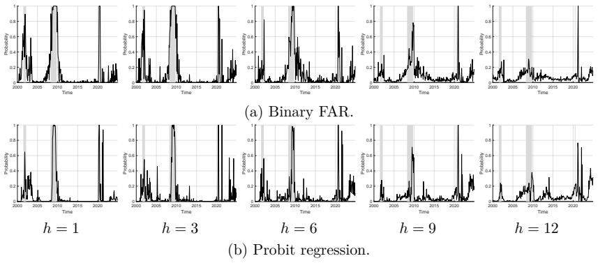
The paper's central claim is that one can replace the continuous response in a factor-augmented forecasting regression with a binary response and estimate it by maximum likelihood, and that the resulting estimators are consistent with a normal limit distribution. The model is $y_{t+h}=\mathbf{1}\{\beta_0+\beta_w'w_t+\beta_f'f_t-\epsilon_{t+h}\ge0\}$ with $x_{it}=\lambda_i'f_t+e_{it}$, and the procedure estimates $f_t$ by principal components, then maximizes the probit log-likelihood using the estimated factors. Theorem 2 is the load-bearing theoretical result: as $N,T\to\infty$ with $\sqrt{T}/N\to0$, $\sqrt{T}(\hat\beta-\tilde H\beta)$ converges in distribution to $N(0,H_0\Sigma_\beta^{-1}\Omega_\beta\Sigma_\beta^{-1}H_0')$, where $\tilde H$ and $H_0$ are rotation matrices that absorb the factor indeterminacy inherent to PCA. The paper further proves that the predicted probability $\Phi_\epsilon(\hat\beta'\tilde z_t)$ converges to the true conditional probability at the rate $O_P(1/\sqrt{N\wedge T})$, and reports simulation and empirical evidence that the model outperforms conventional probit.
Load-bearing premise
The load-bearing premise is that the linear index $\beta'z_t$ lies in a fixed bounded range with probability approaching one and that the error density stays positive on that range; if the estimated factors or predictors can run off to extreme values, the consistency and normality proofs no longer hold.
Editorial extensions
If this is right
- At every horizon considered ($h=1,3,6,9,12$ months), the model's AUC exceeds the conventional probit benchmark in both in-sample and out-of-sample comparisons; for example, out-of-sample AUC at $h=1$ is 0.982 versus 0.898.
- Because $\sqrt{T}(\hat\beta-\tilde H\beta)$ is asymptotically normal, applied users can construct confidence intervals and tests for the coefficients even though the factors are estimated in a first step.
- Predicted recession probabilities are consistent at rate $O_P(1/\sqrt{N\wedge T})$, so adding cross-sectional predictors and more time observations both improve the probability forecasts.
- The factor number can be selected by the paper's information criterion, which is consistent, so the practitioner does not need to know the number of latent factors in advance.
- When some predictors are discrete, the first PCA step can be replaced by a nonlinear maximum-likelihood factor estimator to keep the same framework.
Reading between the lines
- An extension the authors leave implicit is a formal test of the moving-block bootstrap they adopt for inference; a simulation-based coverage study under their DGPs would tell whether the normal approximation in Theorem 2 delivers reliable confidence intervals in small samples.
- The empirical benchmark is a single probit model using eight hand-selected observable proxies; the paper does not compare against probit with penalized high-dimensional predictors, dynamic probit, or model averaging, so the reported performance gap is specific to that benchmark.
- Because the theorems require the linear index to stay in a bounded set, a practical diagnostic would be to track the in-sample and recursively fitted indices for extreme values; nothing in the simulations or application checks this.
- Re-estimating the recession exercise with real-time data vintages and a shorter recursive window would test whether the out-of-sample advantage survives data revisions and structural shifts that actual forecasters face.
Editorial analysis
A structured set of objections, weighed in public.
Referee Report
Summary. The paper proposes a binary-response factor-augmented regression model in which the latent factors are estimated by principal component analysis and the coefficients are estimated by maximum likelihood. The authors establish consistency (Theorem 1), asymptotic normality (Theorem 2), and a rate for predicted probabilities (Theorem 3) under alpha-mixing and other regularity conditions, propose information-criterion selection of the factor number, and describe a moving-block bootstrap for inference. Finite-sample performance is studied through simulations with normal and logistic errors and with serially correlated errors. The empirical application forecasts U.S. recessions using FRED-MD data and compares the proposed binary FAR model with a conventional Probit model that uses eight observable proxies, reporting in-sample and out-of-sample AUC and pseudo-R2 measures. The headline claim is that the binary FAR model consistently outperforms Probit in both exercises.
Significance. If the theoretical and empirical claims hold, the paper would usefully extend the factor-augmented forecasting literature to binary outcomes, where linear least-squares methods can produce out-of-range probabilities and heteroskedastic errors. The paper provides a fully worked MLE theory built on Bai (2003) and Bai and Ng (2002), and it explicitly targets a practically important forecasting problem. The simulation design covers several dependence and error-distribution settings, and the empirical application is policy-relevant. At the same time, the current evidence has important gaps: the reported simulation AUC tables are identical across different DGPs, the out-of-sample design appears to use full-sample information in selecting factors and proxies, and no uncertainty quantification is provided for the empirical AUC comparisons. These issues are addressable, but they currently prevent the paper's central empirical claim from being regarded as established.
major comments (3)
- [Section 3, Tables 3 and 4] Tables 3 and 4 are numerically identical for every entry, including the means, medians, and standard deviations for all combinations of N, T, and DGP panels, even though Example 1 uses normal errors and Example 2 uses logistic errors. This is almost certainly a reporting error, and as printed it cannot support the claim that the AUC results are robust to the error distribution. Please re-run the simulations and report the correct Table 4, or if the numbers are genuinely identical to three decimal places, state that explicitly and explain why.
- [Section 4.6] The out-of-sample exercise is not genuinely ex ante as currently described. The factor count (IC2 = 8) is fixed in Section 4.3 using what appears to be the full 1960-2024 sample, and the eight observable proxies in Table 5 are selected by full-sample marginal R2. In an expanding-window forecast exercise these choices should be re-made using only information available at each forecast origin. In addition, Table 7 reports only point AUCs; no standard errors, confidence intervals, or tests (DeLong, Diebold-Mariano, or other) are provided, so the reported out-of-sample advantage of binary FAR over Probit is not statistically quantified. Please add uncertainty quantification and either justify the fixed choices or implement recursive selection.
- [Section 2.2, Assumption 2.2 and the Section 3 DGP] Assumption 2.2 requires beta' z_t to lie in a fixed compact set Xi_T with probability approaching one and requires inf_{z in Xi_T} phi_epsilon(z) > c > 0. In the Section 3 DGP the latent factors are Gaussian AR(1) processes with standard normal innovations, so the index beta' z_t is unbounded. No sequence of compact intervals can contain an unbounded Gaussian variable with probability approaching one while the normal density is bounded away from zero on the whole interval; the second requirement fails as the interval expands. The simulations therefore appear to violate a condition used in Theorems 1 and 2, and the empirical application does not check the condition either. Please either verify the condition for the simulation design (for example, with bounded factor supports), relax the assumption, or show that the proofs go through under weaker tail conditions.
minor comments (4)
- [Section 4.6] In the second paragraph of Section 4.6, "classshowsification" should be "classification".
- [Appendix A.1, Lemma A.5] The statement of Lemma A.5 uses l''_t(dot u_t), but the proof immediately bounds l'_t(dot u_t); the notation should be aligned so that the lemma and its proof refer to the same derivative.
- [Section 2.2, moving-block bootstrap] In Step 1 of the moving-block bootstrap, definitions such as y*_{(l-1)q+m+h} = y*_{s_l+m+h} use the bootstrap variable on both sides; the right-hand side should be the original sample value, for example y_{s_l+m+h}.
- [Throughout] There are several typos and spacing issues, including "theoretial" in the Introduction, "coefficeints" in Section 3, "through" for the NBER trough in Section 4.1, and the spacing in "A WHMAN" in Table 5; a careful proofreading pass is needed.
Circularity Check
No circularity: the MLE theory and empirical AUC comparisons are self-contained, with only non-load-bearing author-overlap citations.
full rationale
The claimed derivation is not circular. The model is defined by the index β'z_t with z_t = (1, w_t', f_t')' and the binary outcome y_{t+h} = 1{β'z_t − ε_{t+h} ≥ 0}; the likelihood is the standard Bernoulli likelihood with known CDF Φ_ε, and β̂ is the argmax of that likelihood after replacing f_t by PCA estimates. Theorems 1–3 are proven from Assumptions 1–3 using the Bai (2003) and Bai–Ng (2002) PCA rate, Taylor expansions of the log-likelihood, and a conventional sandwich variance Σ_β^{-1}Ω_βΣ_β^{-1}; no parameter, likelihood, or variance is defined in terms of the estimator's limiting distribution, and no prediction is constructed from the fitted values of the benchmark model. The empirical section uses external data (FRED-MD and NBER recession dates) and compares AUCs; the out-of-sample AUCs are not equal by construction to in-sample fits or fitted parameters. Two caveats are correctness concerns rather than circularity: (i) the paper explicitly omits a formal proof for the moving-block bootstrap and for Lemmas A.2–A.3 ('therefore its proof is omitted here'), and (ii) the factor count and observable-proxy choices are selected using the full 1960–2024 sample before the 2000–2024 out-of-sample evaluation, which is potential look-ahead. The only author-overlap citations (Yan and Cheng 2022; Gao et al. 2023) are for related extensions, standard α-mixing conditions, and a technical α-mixing CLT lemma; they are not used as a uniqueness theorem and do not substitute for the paper's own identification argument, so the derivation remains self-contained.
Assumptions & free parameters
free parameters (1)
- Number of factors d0 (empirical) =
8
assumptions (5)
- domain assumption Assumptions 1.1-1.4: strict stationarity, alpha-mixing, moment conditions, and mutual independence of (wt, lambda_i, ft), e_it, and epsilon_t.
- domain assumption Assumption 2.1-2.5: known error distribution, bounded support of the index, smoothness and uniform bounds on the log-likelihood derivatives, and bounded regression coefficients.
- domain assumption Assumption 3.1-3.2: positive definiteness of Sigma_beta and Omega_beta.
- standard math Consistency of the Bai-Ng information criterion for factor number selection.
- domain assumption Moving-block bootstrap consistency.
Cite this review
Pith. "Pith review of Binary Response Forecasting under a Factor-Augmented Framework." pith.science (2026). https://pith.science/paper/KBH4ZIJU
@misc{pith2026250716462,
  author       = {Pith},
  title        = {Pith review of: Binary Response Forecasting under a Factor-Augmented Framework},
  year         = {2026},
  howpublished = {\url{https://pith.science/paper/KBH4ZIJU}},
  note         = {Machine review of arXiv:2507.16462}
}
read the original abstract
In this paper, we propose a novel factor-augmented forecasting regression model with a binary response variable. We develop a maximum likelihood estimation method for the regression parameters and establish the asymptotic properties of the resulting estimators. Monte Carlo simulation results show that the proposed estimation method performs very well in finite samples. Finally, we demonstrate the usefulness of the proposed model through an application to U.S. recession forecasting. The proposed model consistently outperforms conventional Probit regression across both in-sample and out-of-sample exercises, by effectively utilizing high-dimensional information through latent factors.
Figures


Figures from the paper (1 more)
Reference graph
Works this paper leans on
-
[1]
Aastveit, K. A., H. C. Bjørnland, and L. A. Thorsrud (2015). What drives oil prices? emerging versus developed economies. Journal of Applied Econometrics 30 (7), 1013–1028
work page 2015
-
[2]
Ahn, S. C. and A. R. Horenstein (2013). Eigenvalue ratio test for the number of factors. Economet- rica 81 (3), 1203–1227
work page 2013
-
[3]
Audrino, F., A. Kostrov, and J.-P. Ortega (2018). Predicting u.s. bank failures with midas logit models. Journal of Financial and Quantitative Analysis 53 (6), 2685–2713
work page 2018
-
[4]
Bai, J. (2003). Inferential theory for factor models of large dimensions. Econometrica 71 (1), 135–171
work page 2003
-
[5]
Bai, J. (2009). Panel data models with interactive fixed effects. Econometrica 77 (4), 1229–1279
work page 2009
-
[6]
Bai, J. and S. Ng (2002). Determining the number of factors in approximate factor models. Economet- rica 70 (1), 191–221
work page 2002
-
[7]
Bai, J. and S. Ng (2006). Confidence intervals for diffusion index forecasts and inference for factor- augmented regressions. Econometrica 74 (2), 1133–1150
work page 2006
-
[8]
Bai, J. and S. Ng (2008). Forecasting economic time series using targeted predictors. Journal of Econo- metrics 146 (2), 304–317
work page 2008
Show all 59 references
-
[9]
Bai, J. and S. Ng (2013). Principal components estimation and identification of static factors. Journal of Econometrics 176 (1), 18–29
2013
-
[10]
Berge, T. J. (2015). Predicting recessions with leading indicators: Model averaging and selection over the business cycle. Journal of Forecasting 34 (6), 455–471
2015
-
[11]
Bosq, D. (1996). Inequalities for mixing processes, pp. 15–37. New York, NY: Springer US
1996
-
[12]
Masten, and M
Brezigar-Masten, A., I. Masten, and M. Volk (2021). Modeling credit risk with a Tobit model of days past due. Journal of Banking & Finance 122 , 105984
2021
-
[13]
Kelly, A
Bybee, L., B. Kelly, A. Manela, and D. Xiu (2024). Business news and business cycles. The Journal of Finance 79 (5), 3105–3147
2024
-
[14]
Charalambous, C., S. H. Martzoukos, and Z. T. and (2023). A neuro-structural framework for bankruptcy prediction. Quantitative Finance 23 (10), 1445–1464
2023
-
[15]
Chauvet, M. and S. Potter (2005). Forecasting recessions using the yield curve. Journal of Forecast- ing 24 (2), 77–103
2005
-
[16]
Fan, and X
Chen, E., J. Fan, and X. Zhu (2024). Factor augmented matrix regression. Working paper available at https://arxiv.org/abs/2405.17744
2024 arXiv
-
[17]
Hong, and H
Chen, Q., Y. Hong, and H. Li (2024). Time-varying forecast combination for factor-augmented regressions with smooth structural changes. Journal of Econometrics 240 (1), 105693
2024
-
[18]
Cheng, X. and B. E. Hansen (2015). Forecasting with factor-augmented regression: A frequentist model averaging approach. Journal of Econometrics 186 (2), 280–293
2015
-
[19]
Christiansen, C., J. N. Eriksen, and S. V. Møller (2014). Forecasting us recessions: The role of sentiment. Journal of Banking & Finance 49 , 459–468
2014
-
[20]
Djogbenou, A. A. (2021). Model selection in factor-augmented regressions with estimated factors. Econo- metric Reviews 40 (5), 470–503
2021
-
[21]
Ercolani, V. and F. Natoli (2020). Forecasting us recessions: the role of economic uncertainty. Economics 35 letters 193, 109302
2020
-
[22]
Estrella, A. (1998). A new measure of fit for equations with dichotomous dependent variables. Journal of Business & Economic Statistics 16 (2), 198–205
1998
-
[23]
Estrella, A. and F. S. Mishkin (1998). Predicting us recessions: Financial variables as leading indicators. Review of Economics and Statistics 80 (1), 45–61
1998
-
[24]
Estrella, A. and M. Trubin (2006). The yield curve as a leading indicator: Some practical issues. Current issues in Economics and Finance 12 (5)
2006
-
[25]
Fan, J. and Y. Gu (2024). Factor augmented sparse throughput deep relu neural networks for high dimensional regression. Journal of the American Statistical Association 119 (548), 2680–2694
2024
-
[26]
Fan, J. and Q. Yao (2003). Nonlinear Time Series: Nonparametric and Parametric Methods . Springer- Verlag
2003
-
[27]
Feng, C., H. Wang, Y. Han, Y. Xia, and X. M. Tu (2013). The mean value theorem and taylor’s expansion in statistics. The American Statistician 67 (4), 245–248
2013
-
[28]
Fornaro, P. (2016). Forecasting us recessions with a large set of predictors. Journal of Forecasting 35(6), 477–492
2016
-
[29]
Gao, J. (2007). Nonlinear Time Series: Semi– and Non–Parametric Methods . Chapman & Hall/CRC
2007
-
[30]
Gao, J., F. Liu, B. Peng, and Y. Yan (2023). Binary response models for heterogeneous panel data with interactive fixed effects. Journal of Econometrics 235 (2), 1654–1679
2023
-
[31]
Xia, and H
Gao, J., K. Xia, and H. Zhu (2020). Heterogeneous panel data models with cross-sectional dependence. Journal of Econometrics 219 (2), 329–353. Gon¸ calves, S., M. W. McCracken, and B. Perron (2017). Tests of equal accuracy for nested models with estimated factors. Journal of E...
2020
-
[32]
Kelly, and D
Gu, S., B. Kelly, and D. Xiu (2021). Autoencoder asset pricing models. Journal of Econometrics 222 (1), 429–450
2021
-
[33]
Hannadige, S. B., J. Gao, M. J. Silvapulle, and P. S. and (2024). Forecasting a nonstationary time series using a mixture of stationary and nonstationary factors as predictors. Journal of Business & Economic Statistics 42 (1), 122–134
2024
-
[34]
Higgins, A. and K. Jochmans (2025). Inference in dynamic models for panel data using the moving block bootstrap. Working paper available at arXiv:2502.08311
2025 arXiv
-
[35]
Jones, S. (2017). Corporate bankruptcy prediction: a high dimensional analysis. Review of Accounting Studies 22 (3), 1366–1422
2017
-
[36]
Johnstone, and R
Jones, S., D. Johnstone, and R. Wilson (2017). Predicting corporate bankruptcy: An evaluation of alternative statistical frameworks. Journal of Business Finance & Accounting 44 (1-2), 3–34
2017
-
[37]
Urbain, and J
Karabiyik, H., J.-P. Urbain, and J. Westerlund (2019). Cce estimation of factor-augmented regression models with more factors than observables. Journal of Applied Econometrics 34 (2), 268–284
2019
-
[38]
Kauppi, H. and P. Saikkonen (2008). Predicting us recessions with dynamic binary response models. The Review of Economics and Statistics 90 (4), 777–791
2008
-
[39]
Kelly, B. and S. Pruitt (2015). The three-pass regression filter: A new approach to forecasting using many predictors. Journal of Econometrics 186 (2), 294–316
2015
-
[40]
Kim, D., K. Kwon, J. Lee, and S.-G. Lee (2022). Predicting bank failure: Evidence from the US banking 36 sector. Journal of Financial Stability 58 , 100940. K¨ unsch, H. R. (1989). The jackknife and the bootstrap for general stationary observations. The Annals of Statistics , ...
2022
-
[41]
Laitinen, E. K. (1999). Predicting a corporate credit analyst’s risk estimate by logistic and linear models. International Review of Financial Analysis 8 (2), 97–121
1999
-
[42]
Tosasukul, and W
Li, D., J. Tosasukul, and W. Zhang (2020). Nonlinear factor-augmented predictive regression models with functional coefficients. Journal of Time Series Analysis 41 (3), 367–386
2020
-
[43]
Li, F., K. R. Ramesh, and M. Shen (2020). Predicting corporate bankruptcy: What matters? Journal of Accounting, Auditing & Finance 35 (1), 150–176
2020
-
[44]
Zhang, and H
Liu, J., X. Zhang, and H. Xiong (2024). Credit risk prediction based on causal machine learning: Bayesian network learning, default inference, and interpretation. Journal of Forecasting 43 (5), 1625–1660
2024
-
[45]
Liu, W. and E. Moench (2016). What predicts us recessions? International Journal of Forecasting 32(4), 1138–1150
2016
-
[46]
Huang, L
Liu, Y., F. Huang, L. Ma, Q. Zeng, and J. Shi (2024). Credit scoring prediction leveraging interpretable ensemble learning. Journal of Forecasting 43 (2), 286–308
2024
-
[47]
Massacci, D. and G. Kapetanios (2024). Forecasting in factor augmented regressions under structural change. International Journal of Forecasting 40 (1), 62–76
2024
-
[48]
McCracken, M. W. and S. Ng (2016). Fred-md: A monthly database for macroeconomic research.Journal of Business & Economic Statistics 34 (4), 574–589
2016
-
[49]
Ng, E. C. (2012). Forecasting us recessions with various risk factors and dynamic probit models. Journal of Macroeconomics 34 (1), 112–125
2012
-
[50]
Ponka, H. (2017). The role of credit in predicting us recessions. Journal of Forecasting 36 (5), 469–482. Proa˜ no, C. R. and T. Theobald (2014). Predicting recessions with a composite real-time dynamic probit model. International Journal of Forecasting 30 (4), 898–917
2017
-
[51]
Qiu, Y., T. Xie, J. Yu, and Q. Zhou (2020, 06). Forecasting equity index volatility by measuring the linkage among component stocks. Journal of Financial Econometrics 20 (1), 160–186
2020
-
[52]
Silva, D. M., G. H. Pereira, and T. M. Magalh˜ aes (2022). A class of categorization methods for credit scoring models. European Journal of Operational Research 296 (1), 323–331
2022
-
[53]
Stock, J. H. and M. W. Watson (2002). Forecasting using principal components from a large number of predictors. Journal of the American Statistical Association 97 (460), 1167–1179
2002
-
[54]
Swanson, N. R., W. Xiong, and X. Yang (2020). Predicting interest rates using shrinkage methods, real- time diffusion indexes, and model combinations. Journal of Applied Econometrics 35 (5), 587–613
2020
-
[55]
Tu, Y. and S. Wang (2025). Consistent model selection for factor-augmented regressions. Economics Letters 253, 112331
2025
-
[56]
Vrontos, S. D., J. Galakis, and I. D. Vrontos (2021). Modeling and predicting us recessions using machine learning techniques. International Journal of Forecasting 37 (2), 647–671
2021
-
[57]
Wang, F. (2022). Maximum likelihood estimation and inference for high dimensional generalized factor models with application to factor-augmented regressions. Journal of Econometrics 229 (1), 180–200
2022
-
[58]
Cui, and K
Wang, S., G. Cui, and K. Li (2015). Factor-augmented regression models with structural change. Eco- nomics Letters 130 , 124–127. 37
2015
-
[59]
Yan, Y. and T. Cheng (2022). Factor-augmented forecasting regressions with threshold effects. The Econometrics Journal 25 (1), 134–154. C ¸ akmaklı, C. and D. van Dijk (2016). Getting the most out of macroeconomic information for predicting excess stock returns. International ...
2022
Reviewed August 6, 2026 · model on record in the stance chip above.
Discussion (0). Sign in to comment.