REVIEW 5 minor 36 references
Gromov-Hausdorff distance between chromatic metric pairs and stability of the six-pack
T0 review · 0 major / 5 minor · reviewed 2026-08-06 · deepseek-v4-flash
Pith's one-line read A color-constrained Gromov-Hausdorff distance makes the six-pack of persistence diagrams stable.
desk verdict A correct and genuinely useful stability theorem for chromatic persistence; two minor issues don't threaten the core. read the letter →
The pith
A machine-rendered reading of the paper's core claim, the machinery that carries it, and where it could break.
The reading
What carries the argument
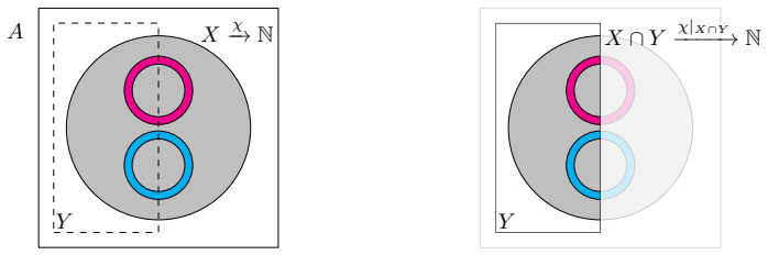
The central object is the $C$-constrained Gromov-Hausdorff distance, defined as half the infimum over pairs $f:A_1\to A_2$, $g:A_2\to A_1$ of $\max\{\operatorname{dis} f, \operatorname{dis} g, \operatorname{codis}(f,g)\}$, where all maps are required to be $C$-constrained: for every $\sigma\in C$, $f(\chi_1^{-1}(\sigma))\subseteq \chi_2^{-1}(\sigma)$. The stability proof is carried by Lemmas 5.2–5.4: a $C(\Gamma)\cup C(\Lambda)$-constrained pair of maps with distortion and codistortion at most $2\varepsilon$ induces, for every radius $\delta$, simplicial maps between the $\Gamma$- and $\Lambda$-subcomplexes of the ambient Čech filtrations, and these maps form interleavings that commute up to contiguity. Homology converts these into genuine $2\varepsilon$-interleavings of the six persistence modules, and the algebraic stability theorem turns those into bottleneck-distance bounds on the persistence diagrams.
What would settle it
Take two finite colored point sets in the plane with $\Lambda = \{\{0\}\}$ and $\Gamma = \{\{0\},\{1\},\{0,1\}\}$, compute $d^{C}_{GH}$ for $C=\{\{0\},\{0,1\}\}$ by the pair-of-maps definition, and compute the six persistence diagrams on a fine discretization, as in Example 5.6; the theorem is false if any instance gives $d_B$ larger than $2\,d^{C}_{GH}$.
Extended reading notes
Core claim
The paper's central claim is that the six-pack is stable with respect to the constrained distance: for finite colored subsets $X_1 \subseteq A_1$ and $X_2 \subseteq A_2$, with $\Lambda \leq \Gamma$ finite-dimensional simplicial complexes on the color set and $C = C(\Gamma) \cup C(\Lambda)$ the union of their sets of maximal faces, each of the six persistence modules — domain, codomain, image, kernel, cokernel, and relative homology built from the inclusions $\check{C}^\Lambda(\chi;A) \hookrightarrow \check{C}^\Gamma(\chi;A)$ — satisfies $d_B(\operatorname{Dgm} U_1, \operatorname{Dgm} U_2) \leq 2\,d^{C}_{GH}((A_1,\chi_1),(A_2,\chi_2))$. The constraining family $C$ is not incidental: it is exactly what guarantees that a $C$-constrained map sends $\Gamma$-colored simplices of the Čech filtration to $\Gamma$-colored simplices at a controlled radius shift (Lemma 5.2).
Load-bearing premise
The whole bound rests on the existence, for nearly equal colored point sets, of two maps that respect exactly the chosen color groupings and have both distortion and codistortion below $2\varepsilon$; if the constraint set is looser or the point sets are infinite, the interleaving construction is not guaranteed and the bottleneck bound can fail.
Editorial extensions
If this is right
- If two finite colored point sets are close in $d^{C}_{GH}$ with $C=C(\Gamma)\cup C(\Lambda)$, then all six persistence diagrams in the six-pack are close in bottleneck distance, with constant 2.
- The ambient Čech persistence diagrams of two finite metric pairs are stable with respect to the induced Gromov-Hausdorff distance for metric pairs (Corollary 5.7).
- The new distance inherits classical characterizations: it can be computed via correspondences or common embeddings, and under compactness it is attained and vanishes exactly for constrained isomorphisms (Theorem 4.9, Theorem 4.13, Corollary 4.20).
- Weaker constraint sets yield smaller distances, so invariants that ignore some color information can be bounded more tightly by choosing weaker constraints (Remark 4.3(iv), Example 4.4).
- The six-pack stability generalizes earlier stability results for metric pairs and for degree-0 image, kernel, and cokernel persistence with Vietoris-Rips filtrations.
Reading between the lines
- The same interleaving-by-contiguity skeleton should transfer to other geometric complexes, such as Vietoris-Rips or Dowker filtrations, since the proof only needs the radius-shift and contiguity lemmas, not the spherical geometry of Čech balls.
- The paper's bracketed conjecture that the persistence diagrams of $(X,\operatorname{rad}_A)$ and of the ambient Čech filtration coincide, if true, would remove the circumradius-attainment hypothesis from the tripod-based proof and extend Corollary 5.7 to all finite metric pairs.
- For labeled point-cloud matching, this suggests a practical recipe: choose the weakest constraint set compatible with the labels an application cares about, compute $d^{C}_{GH}$, and use the six-pack bottleneck distances as certified lower bounds; Example 5.6 shows such lower bounds can be tight.
Editorial analysis
A structured set of objections, weighed in public.
Referee Report
Summary. The paper introduces chromatic metric pairs (A, χ:X→N), C-constrained maps, and a C-constrained Gromov-Hausdorff distance d_C_GH defined by minimizing max{dis f, dis g, codis(f,g)} over C-constrained pairs of maps. It establishes basic properties of this distance, characterizations via C-constrained correspondences and via admissible metrics on disjoint unions, existence of optimal correspondences for C-compact pairs, and stable lower-bound invariants. The central result is Theorem 5.5: for finite X1 and X2 and finite-dimensional simplicial complexes Λ ≤ Γ on N, each of the six persistence modules (domain, codomain, image, kernel, cokernel, relative homology) satisfies dB(Dgm U1, Dgm U2) ≤ 2 d_{C(Γ)∪C(Λ)}_GH((A1, χ1), (A2, χ2)). Corollary 5.7 derives stability for ambient Čech persistence diagrams, and Section 5.3 gives an alternative tripod-based proof under an additional technical assumption.
Significance. The paper supplies a natural and genuinely new distance for colored metric data and proves the first stability theorem for the six-pack with respect to such a distance. The foundational development is careful: the Alexandrov-topology analysis of constraint sets in Section 3.1 is elegant and useful, the computations in Section 4.1 provide sharp worked examples, and the main theorem is a substantial extension of persistence stability to chromatic settings. The proof adapts Chowdhury–Mémoli interleaving techniques and the algebraic stability theorem in a coherent way, and the distance is defined independently of persistence, so there is no circularity. I concur with the stress-test assessment: the flagged issues in Proposition 4.12 and Section 5.3 are real but do not affect the central six-pack stability theorem. The main limitations are the finiteness assumption in Theorem 5.5 and the unresolved question in Section 5.3, both of which are stated explicitly in the manuscript.
minor comments (5)
- [§4.2, proof of Proposition 4.12] The displayed equality 'sup_σ sup_{(y,z)∈R_σ} d(y,z) = sup_{(y,z)∈R} d(y,z)' is false in general, because R also contains the arbitrary correspondence R′ and the supremum over R can be larger. The intended inequality d_C_H(Y,Z) ≤ max{d_H(Y,Z), sup_σ d_H(Y_σ,Z_σ)} can be obtained by choosing R′ and the R_σ with suprema close to the corresponding Hausdorff values, so the statement of the proposition is correct, but the proof as written needs this repair.
- [§5.3, bracketed question after Proposition 5.8] The bracketed sentence 'I suspect that even in the general setting the persistence diagrams of (X, rad_A) and Č(X;A) coincide, don’t they?' is an acknowledged open point inside the alternative proof. Since Corollary 5.7 follows directly from Theorem 5.5, this does not threaten the central claim, but the sentence should be resolved, removed, or converted into an explicit open question.
- [§5.3, proof of Proposition 5.8] In the proof, after choosing a2, the conclusion 'rad_{A2}(π1(σ)) ≤ rad_{A1}(π1(σ)) + dis R + ε' should refer to rad_{A2}(π2(σ)); the same notational slip occurs in the following displayed line.
- [§5.2, proof of Lemma 5.2] The sentence 'we define f_δ ... on the vertex set by setting f_δ(x) = f(x) for every vertex x of Γ' should read 'for every vertex x of Č_δ(X1; A1)' or 'of X1'; as written, it is confusing because Γ has vertices in N and is not the source complex of f_δ.
- [Throughout] There are several typos that should be corrected: 'Gromov-Hausdroff' in Section 2, 'C-cconstrained' in the caption of Figure 13, and 'a constraint set N∈C⊆P(N)' in Example 5.6 should read 'C⊆P(N) with N∈C'. None of these affects the mathematics.
Circularity Check
No significant circularity: the C-constrained Gromov-Hausdorff distance is defined independently, and Theorem 5.5 derives six-pack stability via external algebraic stability and contiguity arguments.
full rationale
The central derivation chain is self-contained against external benchmarks. dC_GH (Definition 4.1) is an independent infimum over C-constrained map pairs, and the six-pack modules (Section 5.1–5.2) are defined from the Cech filtrations and the inclusion Lambda <= Gamma. Theorem 5.5 does not define either quantity in terms of the other; it constructs 2-epsilon-interleavings in Lemma 5.3 (adapting [8, Proposition 15]) and then invokes the algebraic stability theorem [5]. The only author self-citations, [13]/[14], supply the six-pack construction as background and a parenthetical homotopy-equivalence remark, which is not used in the proof of Theorem 5.5. The alternative proof in Section 5.3 has an explicitly flagged gap: '[[I suspect that even in the general setting the persistence diagrams of (X, radA) and C(X;A) coincide, don't they?]]' and requires the circumradius infimum to be attained, but this route is not needed, since Corollary 5.7 follows from Theorem 5.5 by taking Gamma = {{0}} and Lambda = empty. The reversed displayed inequality in the proof of Proposition 4.12 is a proof/correctness typo (the statement is the reverse of the bound just established) and is not central to the stability theorem. No fitted parameter is relabeled as a prediction, and no uniqueness result is imported from the authors' own prior work. Hence the paper's derivation is not circular.
Assumptions & free parameters
assumptions (5)
- standard math ZFC set theory and standard point-set topology
- standard math Pointwise finite-dimensional persistence modules decompose into interval modules (Crawley-Boevey)
- standard math Algebraic stability theorem for q-tame modules (Chazal, Cohen-Steiner, Glisse, Guibas, Oudot)
- domain assumption Finiteness of X1 and X2 in the main stability theorem
- domain assumption The circumradius infimum in equation (8) is attained for every subset
Cite this review
Pith. "Pith review of Gromov-Hausdorff distance between chromatic metric pairs and stability of the six-pack." pith.science (2026). https://pith.science/paper/2DPELB44
@misc{pith2026250717994,
  author       = {Pith},
  title        = {Pith review of: Gromov-Hausdorff distance between chromatic metric pairs and stability of the six-pack},
  year         = {2026},
  howpublished = {\url{https://pith.science/paper/2DPELB44}},
  note         = {Machine review of arXiv:2507.17994}
}
read the original abstract
Chromatic metric pairs consist of a metric space and a coloring function partitioning a subset thereof into various colors. It is a natural extension of the notion of chromatic point sets studied in chromatic topological data analysis. A useful tool in the field is the six-pack, a collection of six persistence diagrams, summarizing homological information about how the colored subsets interact. We introduce a suitable generalization of the Gromov-Hausdorff distance to compare chromatic metric pairs. We show some basic properties and validate this definition by obtaining the stability of the six-pack with respect to that distance. We conclude by discussing its restriction to metric pairs and its role in the stability of the \v{C}ech persistence diagrams.
Figures


Figures from the paper (10 more)




Reference graph
Works this paper leans on
-
[1]
P.K. Agarwal, K. Fox, A. Nath, A. Sidiropoulos, Y. Wang, Computing the Gromov-Hausdorff Dis- tance for Metric Trees, ACM Transactions on Algorithms 14 (2), 1–20 (2018)
work page 2018
-
[2]
Y. Reani, O. Bobrowski, A Coupled Alpha Complex , Journal of Computational Geometry 14 (1) (2023), 221–256, doi:10.20382/jocg.v14i1a9
- [3]
-
[4]
T. Chaplin, H.A. Harrington, U. Tillmann, Grounded Persistent Path Homology: A Stable, Topo- logical Descriptor for Weighted Digraphs , Found. Comput. Math. (2024)
work page 2024
- [5]
- [6]
- [7]
-
[8]
S. Chowdhury, F. M´ emoli, A functorial Dowker theorem and persistent homology of asymmetric networks, Journal of Applied and Computational Topology 2 (1) (2018), 115–175
work page 2018
Show all 36 references
-
[9]
Chowdhury, F
S. Chowdhury, F. M´ emoli,Explicit geodesics in Gromov-Hausdorff space . Electron. Res. Announc. 25, 48–59 (2018)
2018
-
[10]
Cohen-Steiner, H
D. Cohen-Steiner, H. Edelsbrunner, J. Harer, Stability of persistence diagrams , in Proc. 21st ACM Sympos. Comput. Geom., pages 263–271, 2005
2005
-
[11]
Cohen-Steiner, H
D. Cohen-Steiner, H. Edelsbrunner, J. Harer, D. Morozov, Persistent Homology for Kernels, Im- ages, and Cokernels , Proceedings of the Twentieth Annual ACM-SIAM Symposium on Discrete Algorithms, 1011–1020 (2009)
2009
-
[12]
Crawley-Boevey, Decomposition of pointwise finite-dimensional persistence modules , Journal of Algebra and Its Applications 14(5), 1550066 (2015) doi:10.1142/S0219498815500668
W. Crawley-Boevey, Decomposition of pointwise finite-dimensional persistence modules , Journal of Algebra and Its Applications 14(5), 1550066 (2015) doi:10.1142/S0219498815500668
2015 doi
-
[13]
Cultrera di Montesano, O
S. Cultrera di Montesano, O. Draganov, H. Edelsbrunner, M. Saghafian, Chromatic Alpha Com- plexes, Foundations of Data Science, doi:10.3934/fods.2025003 (2024)
2024 doi
-
[14]
Cultrera di Montesano, O
S. Cultrera di Montesano, O. Draganov, H. Edelsbrunner, M. Saghafian, Chromatic Topological Data Analysis, preprint, arXiv:2406.04102 (2024)
2024 arXiv
-
[15]
Dabaghian, F
Y. Dabaghian, F. M´ emoli, L. Frank, G. Carlsson, A Topological Paradigm for Hippocampal Spatial Map Formation Using Persistent Homology , PLoS Comput Biol 8(8): e1002581 (2012). 26
2012
-
[16]
Edelsbrunner and J
H. Edelsbrunner and J. Harer, Computational topology: an introduction , American Mathematical Soc. (2010)
2010
-
[17]
D. A. Edwards, The structure of superspace , published in: Studies in Topology, Academic Press, 1975
1975
-
[18]
Fajstrup, B.T
L. Fajstrup, B.T. Fasy, W. Li, L. Mezrag, T. Rask, F. Tombari, ˇZ. Urbanˇ ciˇ c,Gromov-Hausdorff distance for directed spaces, preprint, arXiv:2408.14394 (2024)
2024
-
[19]
Gabriel, Unzerlegbare Darstellungen I , Manuscripta Math 6, 71–103 (1972), doi:10.1007/BF01298413
P. Gabriel, Unzerlegbare Darstellungen I , Manuscripta Math 6, 71–103 (1972), doi:10.1007/BF01298413
1972 doi
-
[20]
G´ omez, M
A.A. G´ omez, M. Che,Gromov-Hausdorff convergence of metric pairs and metric tuples , Differential Geometry and its Applications, 94, (2024), 102135
2024
-
[21]
Gromov, Structures M´ etriques pour les Vari´ et´ es Riemanniennes(J
M. Gromov, Structures M´ etriques pour les Vari´ et´ es Riemanniennes(J. Lafontaine and P. Pansu, eds.), Textes Math´ ematiques, 1, CEDIC, Paris, 1981
1981
-
[22]
M. I. Kadets, Note on the gap between subspaces , Funkts. Anal. Prilozhen. 9 (1975), no. 2, 73–74; English transl. in Funct. Anal. Appl. 9 (1975), 156–157
1975
-
[23]
N. J. Kalton, M. I. Ostrovskii, Distances between Banach spaces , Forum Mathematicum, 11(1) (1999), 17–48, doi:10.1515/form.11.1.17
1999 doi
-
[24]
Surveys 20: 837-896 (2023)
Ali Khezeli, A unified framework for generalizing the Gromov-Hausdorff metric , Probab. Surveys 20: 837-896 (2023)
2023
-
[25]
S. Lim, F. M´ emoli, O.B. Okutan, Vietoris-Rips persistent homology, injective metric spaces, and the filling radius , Algebraic & Geometric Topology 24, no. 2 (2024), 1019–1100
2024
-
[26]
M´ emoli,Some properties of Gromov-Hausdorff distances , Discrete & Computational Geometry 48 (2) (2012), 416–440
F. M´ emoli,Some properties of Gromov-Hausdorff distances , Discrete & Computational Geometry 48 (2) (2012), 416–440
2012
-
[27]
M´ emoli,A distance between filtered spaces via tripods , preprint, arXiv:1704.03965 (2017)
F. M´ emoli,A distance between filtered spaces via tripods , preprint, arXiv:1704.03965 (2017)
2017 arXiv
-
[28]
M´ emoli, G
F. M´ emoli, G. Sapiro,A Theoretical and Computational Framework for Isometry Invariant Recog- nition of Point Cloud Data , Found. Comput. Math. 313–347 (2005)
2005
-
[29]
J. R. Munkres, Elements of Algebraic Topology, vol. 7. Addison-Wesley, Reading (1984)
1984
-
[30]
Patra, J.R.A
B. Patra, J.R.A. Moniz, S. Garg, M.R. Gormley, G. Neubig, Bilingual Lexicon Induction with Semi-supervision in Non-Isometric Embedding Spaces , Proceedings of the 57th Conference of the Association for Computational Linguistics (2019) 184–193
2019
-
[31]
Petersen, Riemannian Geometry, Springer, New York (1998)
P. Petersen, Riemannian Geometry, Springer, New York (1998)
1998
-
[32]
Stolz, J
B.J. Stolz, J. Dhesi, J.A. Bull, et al., Relational Persistent Homology for Multispecies Data with Application to the Tumor Microenvironment , Bull Math Biol 86, 128 (2024)
2024
-
[33]
Schmiedl, Computational aspects of the Gromov-Hausdorff distance and its application in non- rigid shape matching , Discrete Comput
F. Schmiedl, Computational aspects of the Gromov-Hausdorff distance and its application in non- rigid shape matching , Discrete Comput. Geom. 57, 4 (2017), 854–880
2017
-
[34]
Torras-Casas, R
´A. Torras-Casas, R. Gonzalez-Diaz, Properties and Stability of Persistence Matching Diagrams , arXiv:2409.14954 (2024)
2024 arXiv
-
[35]
A. A. Tuzhilin, Lectures on Hausdorff and Gromov-Hausdorff Distance Geometry , The course was given at Peking University, Fall 2019, arXiv:2012.00756
2019 arXiv
-
[36]
Zava, The stabilty of the q-hyperconvex hull of a quasi-metric space, preprint, arXiv:2208.10619
N. Zava, The stabilty of the q-hyperconvex hull of a quasi-metric space, preprint, arXiv:2208.10619. Inria Centre at Universit´ e Cˆ ote d’Azur ondrej.draganov@inria.fr University of Vienna sophie.rosenmeier@univie.ac.at Institute of Science and Technology Austria (ISTA) nicol...
Reviewed August 6, 2026 · model on record in the stance chip above.
Discussion (0). Continue with ORCID to comment.