A Simple and Robust Weak Galerkin Method for the Brinkman Equations on Non-Convex Polytopal Meshes

Chunmei Wang; Shangyou Zhang

REVIEW 3 major objections 5 minor 37 references

A Simple and Robust Weak Galerkin Method for the Brinkman Equations on Non-Convex Polytopal Meshes

T0 review · 3 major / 5 minor · reviewed 2026-08-15 · deepseek-v4-flash

Challenge this review Re-run · record.json Download PDF Read on arXiv ↗ Review JSON

Pith's one-line read The paper proves that a stabilizer-free weak Galerkin finite element method achieves optimal-order convergence for the Brinkman equations on general polytopal meshes, including non-convex elements.

desk verdict A clean extension of stabilizer-free WG to Brinkman, but the non-convex analysis leans on unproved companion lemmas and the experiments never test the theory or the claimed Darcy/Stokes robustness. read the letter →

arxiv 2507.18896 v1 pith:BVCBBFJM submitted 2025-07-25 math.NA cs.NA

Chunmei Wang , Shangyou Zhang This is my paper · ORCID

classification math.NAcs.NA MSC 65N3065N1565N1265N20

keywords weakGalerkinStabilizer-Freegradientdivergencebubblefunctionsnon-convexpolytopalmeshesBrinkmanequations

verification ladder T0 review T1 audit T2 compute T3 formal

The pith

A machine-rendered reading of the paper's core claim, the machinery that carries it, and where it could break.

The reading

The paper's central claim is that the Brinkman equations—the model that blends Stokes flow in free regions with Darcy flow in porous media—can be solved accurately by a weak Galerkin finite element scheme that contains no explicit stabilization term. The scheme is shown to work on general polytopal meshes whose cells may be non-convex polygons or polyhedra, a case earlier stabilizer-free WG methods left out. If the proof is right, simulations of flow in fractured or vuggy porous media get a simpler discretization with the same optimal accuracy as stabilized schemes, since the stabilizer is replaced by a higher-degree polynomial weak gradient. The central result is that the discrete velocity and pressure errors are $O(h^k)$ in the discrete $H^1$ norm, and the velocity error is $O(h^{k+1})$ in $L^2$, where $k$ is the polynomial degree of the velocity approximation.

What carries the argument

The load-bearing construction is the element bubble function. For a polytopal cell $T$ with $N$ edges or faces $e_1,\dots,e_N$, each with a linear function $l_i$ vanishing on $e_i$, the non-convex case uses $\Phi_B = l_1^2 l_2^2 \cdots l_N^2 \in P_{2N}(T)$, scaled to be one at the barycenter and uniformly positive on a subregion $\hat T$; the discrete weak gradient is then taken in $[P_r(T)]^{d\times d}$ with $r=2N+k-1$ (with the linear-product variant $r=N+k-1$ in the convex case). The bubble product enables the recovery bound $\|\nabla v_0\|_T \le C \|\nabla_w v\|_T$ on non-convex elements, which yields the norm equivalence between $\|\cdot\|_{1,h}$ and $\||\cdot\||$, and that equivalence feeds every subsequent step: the inf-sup condition, the error equation, and the $O(h^k)$ and $O(h^{k+1})$ bounds.

What would settle it

Take a non-convex polygonal cell with one re-entrant angle approaching $360^\circ$, keep its diameter fixed, and compute $\sup_v \|\nabla v_0\|_T/\|\nabla_w v\|_T$ over the discrete space for $k=1$; if this supremum grows without bound as the angle tends to $360^\circ$, the central recovery lemma fails and the optimal error estimates cannot hold uniformly.

Watch

Extended reading notes

Core claim

The paper's central claim is that Algorithm 3.1, which computes the weak gradient in $[P_r(T)]^{d\times d}$ with $r=2N+k-1$ on non-convex cells (or $r=N+k-1$ on convex cells) and uses no stabilizer, produces a unique discrete solution of the Brinkman problem and satisfies the error estimate $\|u-u_h\|_{\text{energy}} + \|p-p_h\| \le C h^k (\|u\|_{k+1} + \|p\|_k)$, together with the $L^2$ velocity bound $\|u-u_0\| \le C h^{k+1}(\|u\|_{k+1}+\|p\|_k)$. The proof constructs bubble functions on each polytopal element to establish a norm equivalence between the discrete $H^1$-type norm and the weak-gradient norm, derives the inf-sup condition for the mixed formulation, obtains the error equation with consistency terms, and bounds those terms by projection approximation estimates.

Load-bearing premise

The whole proof rests on a lemma borrowed from a companion paper that is not proved or tested here: on every non-convex polytopal element the bubble product $l_1^2\cdots l_N^2$ is uniformly positive on some subregion with a constant independent of the element shape, so the recovery bound $\|\nabla v_0\|_T\le C\|\nabla_w v\|_T$ holds with a fixed $C$.

Editorial extensions

If this is right

The scheme eliminates the explicit stabilizer term, so the global stiffness matrix keeps the size and sparsity of a standard WG discretization while implementation simplifies.
Meshes with non-convex polygons or polyhedra can be used as-is, without convexity preprocessing, so arbitrary polytopal partitions from domain decomposition or mesh generators are admissible.
For velocity polynomials of degree $k$ and pressure polynomials of degree $k-1$, the method delivers $O(h^k)$ errors in the discrete energy norm and in pressure, and $O(h^{k+1})$ for velocity in $L^2$, whenever the exact solution has the stated Sobolev regularity.
The same mixed framework covers both Stokes-dominated and Darcy-dominated regimes, so a single code can handle a Brinkman problem as the permeability $\kappa$ varies, at least in the constant-$\kappa$ case analyzed.
The duality argument shows that the $L^2$ velocity error converges one order faster under the standard elliptic-regularity assumption.

Reading between the lines

Editorial extensions of the paper, not claims the author makes directly.

The paper's theory requires $r=2N+k-1$ on non-convex cells, but the experiments use only $r=k+1$, $k+2$, or $k+3$ and still show optimal rates; a plausible reading is that the theoretical degree is a very safe overestimate and the true requirement is much weaker.
The unproved recovery lemma from the companion paper is the single step that ties the whole proof together; proving it directly, or testing it on the actual meshes used in the experiments, would either close the gap or reveal a shape-dependent constant.
Because only the weak-gradient/weak-divergence structure and the inf-sup condition are used, the construction should carry over to variable permeability tensors and to other coupled Stokes–Darcy systems, although the paper itself assumes constant $\kappa$.
A concrete prediction of the analysis is that on a fixed non-convex mesh the convergence order should not change once $r$ is large enough; the error constant may decrease, but the rate is governed by $k$.

Share X Bluesky LinkedIn Reddit HN

Signed reviews

No signed human review yet.

Editorial analysis

A structured set of objections, weighed in public.

Desk editor's note, referee report, and a circularity audit.

Desk Editor's Note

read the letter

The stress-test note goes too far on one detail but is right on the main structural issues. The specific worry about the affine extension of vb is not valid: orthogonal projection onto the face hyperplane is an affine map, so composing with the face polynomial gives a polynomial on the whole element, and the test function φ = (vb−v0)·n φ_ei lands in P_{2N+k−2}, which is inside the discrete weak-gradient space P_{2N+k−1}. That step in Lemma 4.3 is fine.

What is actually new: this is the first stabilizer-free WG scheme for the Brinkman equations on general polytopal meshes, including non-convex elements. The κ^{-1} term is absorbed into the energy norm without introducing new difficulties, and the a priori error analysis is a clean, standard extension of the authors' Stokes framework. The numerical tables show optimal convergence rates on convex and non-convex meshes for k=1..4, which is credible evidence that the method works in practice.

The soft spots are real, and they are exactly where the reader put them. First, the norm equivalence (Lemma 4.3) rests entirely on Lemma 4.1 and Lemma 4.2, which are imported from the authors' own companion papers [16] and [30] without proofs or even precise statements. For a standalone paper, that is a heavy dependency, especially since the non-convex case is the advertised novelty. Second, the inf-sup proof in Lemma 4.5 contains a literal placeholder citation "[?, ?, ?, ?, ?]"; the argument itself is plausible, but the reference gap is sloppy and needs fixing. Third, and most importantly, the numerical experiments use r = k+1, k+2, k+3 while the theory on non-convex elements demands r = 2N+k−1. On the tested meshes that means the experiments never actually exercise the regime the analysis covers. Moreover, every experiment uses κ = 1, so the abstract's claim of robustness across Stokes- and Darcy-dominated flows is never demonstrated; there are no variable-permeability tests and no Darcy-limit or Stokes-limit checks.

This is not a desk-reject case. The paper is a legitimate extension of a working method, the analysis is coherent conditional on the companion lemmas, and the numerical results are useful. The right outcome is peer review with referees who will demand either proofs or full statements of the bubble-function lemmas, a proper inf-sup citation, and at least one experiment with spatially varying κ or with κ driving the problem into the Darcy regime. For researchers in weak Galerkin methods or polytopal finite elements, the paper is worth reading and worth citing as an extension, but the non-convex theory should be treated as inherited rather than established here.

Referee Report

3 major / 5 minor

Summary. The paper proposes a stabilizer-free weak Galerkin (WG) method for the Brinkman equations on polytopal meshes, including non-convex polytopal elements. The velocity trial and test space is piecewise P_k in element interiors and on faces, the pressure space is piecewise P_{k-1}, and the discrete weak gradient is computed in a space P_r with r=2N+k-1 for non-convex elements and r=N+k-1 for convex elements. Existence and uniqueness of the discrete solution are established through a bubble-function-based norm equivalence and an inf-sup condition. Optimal a priori error estimates are claimed in the discrete H^1 norm (Theorem 6.5) and the L^2 norm (Theorem 7.1), with rates h^k and h^{k+1}, respectively. Numerical experiments on triangular, non-convex polygonal, tetrahedral, and non-convex polyhedral meshes report optimal convergence rates for r=k+1, k+2, and k+3.

Significance. The proposed scheme is potentially significant because it removes explicit stabilizers, has a simple implementation, and aims to cover non-convex polytopal meshes, a setting that is uncommon in the stabilizer-free WG literature. The analytical framework is standard once the norm equivalence Lemma 4.3 is granted, and the paper does provide a full error-equation analysis and a conventional duality argument. The manuscript would be strengthened by making the proof of the non-convex norm equivalence self-contained and by running experiments at the polynomial degrees required by the theory; without those additions the central non-convex claim remains conditional.

major comments (3)

[§4, Lemma 4.3 and Eq. (4.7)] The proof of the norm equivalence is load-bearing for every subsequent result, but as written it is incomplete for non-convex elements. The displayed test function φ=(v_b-v0)^T n φ_{e_i} is scalar-valued, whereas the test functions in (2.2) are d×d matrix polynomials; the intended object is presumably the rank-one matrix (v_b-v0)n^T φ_{e_i}. More importantly, the extension v_b(X)=v_b(Proj_{e_i}(X)) is asserted with only 'a suitable extension' when Proj_{e_i}(X)∉e_i, and it is not demonstrated that the resulting matrix-valued test function lies in [P_r(T)]^{d×d} or that the bound ∥φ∥_T^2≤C h_T∫_{e_i}|v_b-v0|^2 ds holds; that bound is imported as Lemma 4.2 from [30] without proof. Since Lemma 4.3 supplies the lower bound in the norm equivalence, which feeds the inf-sup condition (4.12) and hence Theorems 6.5 and 7.1, this gap must be closed in the present manuscript.
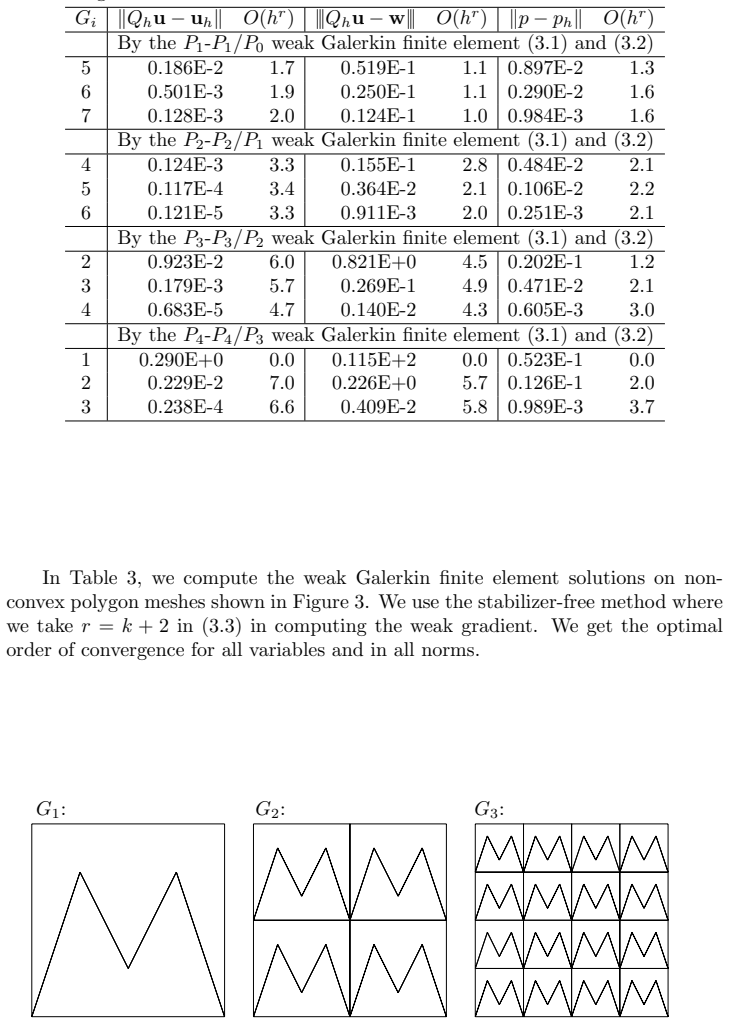
[§8, Tables 1–9] The numerical experiments never use the polynomial degrees required by the theory. Remark 4.1 and Lemma 4.1 require r=2N+k-1 for non-convex elements and r=N+k-1 for convex elements, but the computations use r=k+1, k+2, and k+3 throughout. For the non-convex polygonal meshes of Figures 2–4 with N≥4, this is far below the required degree (e.g., r=2N+k-1≥k+7 for k=1 and N=4), and even Table 1 on triangles uses r=k+1, below the convex requirement k+2. The tables therefore do not validate the central non-convex error estimates. Please either add experiments at the theoretically required degrees or prove the error estimates for the smaller degrees actually used.
[§4, Lemma 4.1 and Remark 4.1] The main a priori estimates depend on Lemma 4.1, which is cited from the companion paper [16] and is not proved or tested here. This lemma asserts a uniform bound ∥∇v0∥_T≤C∥∇w v∥_T for the specific choice r=2N+k-1 (non-convex) or r=N+k-1 (convex). Because the assertion is parameter-free and non-obvious for non-convex polytopes, the manuscript should either include a proof of this lemma, or state the precise hypotheses under which it holds and explain why the companion paper establishes it in the form needed here.

minor comments (5)

[§4, Lemma 4.5] The proof contains the placeholder citation '(see, e.g., [ ?, ?, ?, ?, ?])'; please replace it with concrete references for the surjectivity of the divergence operator from H^1_0(Ω) to L^2_0(Ω).
[§6, Theorem 6.5 proof] In the estimates of I2 and I3, the displayed bounds use ∥p∥_{k+1} while the theorem statement and the final result use ∥p∥_k; this appears to be a typo and should be corrected.
[§4, Eq. (4.7)] The notation φ is reused for the test function and for the bubble function φ_{e_i}; please use distinct symbols for clarity.
[§6, Lemma 6.1] The range 1≤n≤2N+k-1 should be stated separately for convex elements, where the projection degree is N+k-1, or restricted to n=k, which is the value actually used in the paper.
[§8, figure captions] Several figure captions call the meshes 'triangular' even though Figures 2–4, 6–9 display non-convex polygonal or polyhedral meshes; please correct the captions.

Circularity Check

0 steps flagged · score 2.0 of 10

No circular reduction found; central estimates are derived from cited companion lemmas that are parameter-free external support, with non-circular completeness gaps.

full rationale

The central claims (Theorems 6.5 and 7.1) are the discrete H^1 and L^2 error estimates for the Stabilizer-Free WG scheme. Once the norm equivalence (4.6), the inf-sup condition (4.12), and the approximation properties (Lemmas 6.1-6.4) are granted, the proofs are standard and do not reintroduce the target estimate as an input. The norm equivalence itself rests on Lemma 4.1 and Lemma 4.2, both cited from the same authors' prior works ([16], [30]) rather than proved in this paper. These are parameter-free stated inequalities with explicit polynomial-degree conditions (for example, 'r = 2N + k - 1 as stated in Lemma 4.1'), and neither statement contains the Brinkman error estimate; under the review rules they count as independent evidence, not as circular inputs. No fitted parameter is renamed as a prediction, and no equation reduces by construction to an earlier equation. Two non-circular weaknesses are flagged. First, the proof of Lemma 4.3 contains an unproved extension step: 'we extend the function vb, initially defined only on the (d-1)-dimensional face ei, to the full d-dimensional element T ... vb(X) = vb(Projei(X)) ... When Projei(X) /∈ ei, vb is taken as a suitable extension', without showing the resulting test function lies in the required polynomial space [P_r(T)]^{d×d}; this is a gap in the lemma's proof, not a circular step. Second, Lemma 4.5's continuous inf-sup reference is literally missing: '(see, e.g., [?, ?, ?, ?, ?])', and the numerical experiments use r = k+1, k+2, k+3 rather than the r = 2N+k-1 required by Remark 4.1, so the non-convex theoretical regime is not experimentally exercised. These are completeness and validation concerns. The score of 2 reflects the load-bearing same-author citations and unproven imported lemmas; there is no self-definitional, fitted-input, ansatz-import, or renaming circularity.

Assumptions & free parameters 0 free parameters · 5 assumptions · 0 invented entities

The central proofs rely on bubble-function bounds and mesh-regularity assumptions imported, mostly by citation, from the authors' earlier papers, plus one standard functional-analysis fact and a standard duality regularity assumption. There are no fitted constants: all constants in the estimates are generic and independent of h.

assumptions (5)

domain assumption Bubble recovery bound: for a non-convex polytopal element T with N faces, the product of squared face-linear functions Phi_B = l_1^2...l_N^2 is positive on a subregion of T and zero on the boundary, yielding ||grad v0||_T <= C ||grad_w v||_T for weak-gradient degree r = 2N+k-1 (Lemma 4.1).
Cited from [16] by the same authors; not proved in this text. The uniform lower bound rho0 on a subregion of every shape-regular non-convex polytope is assumed rather than established.
domain assumption Edge/face bubble function phi_ei = product over k != i of l_k^2 has a subregion of ei where it is bounded below, and extends to T with ||phi||_T <= C h_T^{1/2} (integral over ei of |vb-v0|^2 ds)^{1/2} (Lemma 4.2).
Cited from [30] by the same authors; used in Lemma 4.3 to control the boundary gap h_T^{-1}||vb-v0||.
domain assumption Shape regularity of polytopal meshes as in [27].
Trace inequalities (4.1)-(4.2) and inverse inequalities are invoked from [27] under a shape-regularity condition that is not restated for non-convex polytopes.
standard math Continuous inf-sup for the divergence operator on Omega, giving the existence of v-bar in [H^1_0(Omega)]^d with (div v-bar, zeta)/||v-bar||_1 >= C||zeta|| for all zeta in L2_0.
Invoked in Lemma 4.5 with the placeholder citation '[?, ?, ?, ?, ?]'.
domain assumption Dual problem regularity: ||w||_2 + ||q||_1 <= C||E0|| in (7.2).
Standard on convex domains; stated as an assumption for the L2 error estimate and not proved in the paper.

how reviews work

0 comments

Cite this review

Pith. "Pith review of A Simple and Robust Weak Galerkin Method for the Brinkman Equations on Non-Convex Polytopal Meshes." pith.science (2026). https://pith.science/paper/BVCBBFJM

@misc{pith2026250718896,
  author       = {Pith},
  title        = {Pith review of: A Simple and Robust Weak Galerkin Method for the Brinkman Equations on Non-Convex Polytopal Meshes},
  year         = {2026},
  howpublished = {\url{https://pith.science/paper/BVCBBFJM}},
  note         = {Machine review of arXiv:2507.18896}
}

read the original abstract

This paper presents a novel Stabilizer-Free weak Galerkin (WG) finite element method for solving the Brinkman equations without the need for conventional stabilization techniques. The Brinkman model, which mathematically blends features of both the Stokes and Darcy equations, describes fluid flow in multi-physics environments, particularly in heterogeneous porous media characterized by spatially varying permeability. In such settings, flow behavior may be governed predominantly by Darcy dynamics in certain regions and by Stokes dynamics in others. A central difficulty in this context arises from the incompatibility of standard finite element spaces: elements stable for the Stokes equations typically perform poorly for Darcy flows, and vice versa. The primary challenge addressed in this study is the development of a unified numerical scheme that maintains stability and accuracy across both flow regimes. To this end, the proposed WG method demonstrates a robust capacity to resolve both Stokes- and Darcy-dominated flows through a unified framework. The method supports general finite element partitions consisting of convex and non-convex polytopal elements, and employs bubble functions as a critical analytical component to achieve stability and convergence. Optimal-order error estimates are rigorously derived for the WG finite element solutions. Additionally, a series of numerical experiments is conducted to validate the theoretical findings, illustrating the method's robustness, reliability, flexibility, and accuracy in solving the Brinkman equations.

Figures

Figures reproduced from arXiv: 2507.18896 by the authors.

**Figure 1.** Gi ∥Qhu − uh∥ O(h r ) |||Qhu − w||| O(h r ) ∥p − ph∥ O(h r ) By the P1-P1/P0 weak Galerkin finite element (3.1) and (3.2) 5 0.317E-3 1.9 0.185E-1 1.0 0.850E-2 0.9 6 0.808E-4 2.0 0.926E-2 1.0 0.431E-2 1.0 7 0.203E-4 2.0 0.463E-2 1.0 0.216E-2 1.0 By the P2-P2/P1 weak Galerkin finite element (3.1) and (3.2) 5 0.474E-5 3.1 0.106E-2 2.0 0.521E-3 2.0 6 0.573E-6 3.0 0.267E-3 2.0 0.129E-3 2.0 7 0.708E-7 3.0 0.668E-4 2.0 0.3… view at source ↗

**Figure 2.** The non-convex polygon meshes for the computation in [PITH_FULL_IMAGE:figures/full_fig_p022_2.png] view at source ↗

Figures from the paper (13 more)

**Figure 2.** Figure 2: Gi ∥Qhu − uh∥ O(h r ) |||Qhu − w||| O(h r ) ∥p − ph∥ O(h r ) By the P1-P1/P0 weak Galerkin finite element (3.1) and (3.2) 5 0.186E-2 1.7 0.519E-1 1.1 0.897E-2 1.3 6 0.501E-3 1.9 0.250E-1 1.1 0.290E-2 1.6 7 0.128E-3 2.0 0.124E-1 1.0 0.984E-3 1.6 By the P2-P2/P1 weak Gal…

**Figure 3.** Figure 3: The non-convex polygon meshes for the computation in [PITH_FULL_IMAGE:figures/full_fig_p023_3.png]

**Figure 3.** Figure 3: Gi ∥Qhu − uh∥ O(h r ) |||Qhu − w||| O(h r ) ∥p − ph∥ O(h r ) By the P1-P1/P0 weak Galerkin finite element (3.1) and (3.2) 5 0.536E-3 1.9 0.501E-1 1.0 0.299E-2 1.3 6 0.137E-3 2.0 0.251E-1 1.0 0.124E-2 1.3 7 0.343E-4 2.0 0.125E-1 1.0 0.578E-3 1.1 By the P2-P2/P1 weak Gal…

**Figure 4.** Figure 4: The non-convex polygon meshes for the computation in [PITH_FULL_IMAGE:figures/full_fig_p024_4.png]

**Figure 4.** Figure 4: Gi ∥Qhu − uh∥ O(h r ) |||Qhu − w||| O(h r ) ∥p − ph∥ O(h r ) By the P1-P1/P0 weak Galerkin finite element (3.1) and (3.2) 5 0.312E-3 2.0 0.344E-1 1.0 0.837E-2 1.0 6 0.787E-4 2.0 0.172E-1 1.0 0.420E-2 1.0 7 0.197E-4 2.0 0.863E-2 1.0 0.210E-2 1.0 By the P2-P2/P1 weak Gal…

**Figure 5.** Figure 5: The triangular meshes for the computation in [PITH_FULL_IMAGE:figures/full_fig_p026_5.png]

**Figure 6.** Figure 6: The triangular meshes for the computation in [PITH_FULL_IMAGE:figures/full_fig_p027_6.png]

**Figure 7.** Figure 7: The triangular meshes for the computation in [PITH_FULL_IMAGE:figures/full_fig_p027_7.png]

**Figure 7.** Figure 7: Gi ∥Qhu − uh∥ O(h r ) |||Qhu − w||| O(h r ) ∥p − ph∥ O(h r ) By the P1-P1/P0 weak Galerkin finite element (3.1) and (3.2) 2 0.116E+0 1.51 0.366E+1 0.00 0.566E+0 0.00 3 0.253E-1 2.20 0.142E+1 1.36 0.220E+0 1.36 4 0.533E-2 2.25 0.433E+0 1.71 0.678E-1 1.70 By the P2-P2/P1…

**Figure 8.** Figure 8: The triangular meshes for the computation in [PITH_FULL_IMAGE:figures/full_fig_p028_8.png]

**Figure 8.** Figure 8: Gi ∥Qhu − uh∥ O(h r ) |||Qhu − w||| O(h r ) ∥p − ph∥ O(h r ) By the P1-P1/P0 weak Galerkin finite element (3.1) and (3.2) 2 0.879E-1 1.97 0.333E+1 0.00 0.512E+0 0.22 3 0.317E-1 1.47 0.130E+1 1.36 0.315E+0 0.70 4 0.748E-2 2.08 0.434E+0 1.58 0.116E+0 1.44 By the P2-P2/P1…

**Figure 9.** Figure 9: The triangular meshes for the computation in [PITH_FULL_IMAGE:figures/full_fig_p029_9.png]

**Figure 9.** Figure 9: Gi ∥Qhu − uh∥ O(h r ) |||Qhu − w||| O(h r ) ∥p − ph∥ O(h r ) By the P1-P1/P0 weak Galerkin finite element (3.1) and (3.2) 2 0.164E+0 0.77 0.858E+1 0.00 0.320E+1 0.00 3 0.969E-1 0.76 0.350E+1 1.29 0.109E+1 1.56 4 0.362E-1 1.42 0.122E+1 1.52 0.248E+0 2.13 By the P2-P2/P1…

Discussion (0). Continue with ORCID to comment.

Reference graph

Works this paper leans on

37 extracted references · 25 canonical work pages

[16]

W ang, Auto-Stabilized Weak Galerkin Finite Element Methods on Polytopal Meshes with- out Convexity Constraints , arXiv:2408.11927

C. W ang, Auto-Stabilized Weak Galerkin Finite Element Methods on Polytopal Meshes with- out Convexity Constraints , arXiv:2408.11927

arXiv
[30]

W ang and S

C. W ang and S. Zhang , Auto-Stabilized Weak Galerkin Finite Element Methods for Stokes Equations on Non-Convex Polytopal Meshes , Journal of Computational Physics, vol. 533, 114006, 2025

work page 2025
[1]

Badia and R

S. Badia and R. Codina , Unified stabilized finite element formulations for the Stokes and the Darcy problems, SIAM J. Numer. Anal., 47 (2009), 1971-2000

work page 2009
[2]

Knn and R

J. Knn and R. Stenberg , H(div)-conforming finite elements for the Brinkman problem , Math. Models and Meth. Applied Sciences, 11 (2011), 2227-2248

work page 2011
[3]

Mardal, X

K. Mardal, X. Tai, and R. Winther , A Robust finite element method for Darcy-Stokes flow, SIAM J. Numer. Anal., 40 (2002), 1605-1631

work page 2002
[4]

S. Cao, C. W ang and J. W ang , A new numerical method for div-curl Systems with Low Regularity Assumptions, Computers and Mathematics with Applications, vol. 144, pp. 47-59, 2022

work page 2022
[5]

D. Li, Y. Nie, and C. W ang , Superconvergence of Numerical Gradient for Weak Galerkin Finite Element Methods on Nonuniform Cartesian Partitions in Three Dimensions , Com- puters and Mathematics with Applications, vol 78(3), pp. 905-928, 2019

work page 2019
[6]

D. Li, C. W ang and J. W ang , An Extension of the Morley Element on General Polytopal Partitions Using Weak Galerkin Methods, Journal of Scientific Computing, 100, vol 27, 2024

work page 2024

Show all 37 references

[7]

D. Li, C. W ang and S. Zhang , Weak Galerkin methods for elliptic interface problems on curved polygonal partitions, Journal of Computational and Applied Mathematics, pp. 115995, 2024

2024
[8]

D. Li, C. W ang, J. W ang and X. Ye , Generalized weak Galerkin finite element methods for second order elliptic problems , Journal of Computational and Applied Mathematics, vol. 445, pp. 115833, 2024

2024
[9]

D. Li, C. W ang, J. W ang and S. Zhang , High Order Morley Elements for Biharmonic Equations on Polytopal Partitions , Journal of Computational and Applied Mathematics, Vol. 443, pp. 115757, 2024

2024
[10]

D. Li, C. W ang and J. W ang , Curved Elements in Weak Galerkin Finite Element Methods , Computers and Mathematics with Applications, Vol. 153, pp. 20-32, 2024

2024
[11]

D. Li, C. W ang and J. W ang , Generalized Weak Galerkin Finite Element Methods for Bi- harmonic Equations, Journal of Computational and Applied Mathematics, vol. 434, 115353, 2023

2023
[12]

D. Li, C. W ang, and J. W ang , Superconvergence of the Gradient Approximation for Weak Galerkin Finite Element Methods on Rectangular Partitions , Applied Numerical Mathemat- ics, vol. 150, pp. 396-417, 2020

2020
[13]

W ang, A Preconditioner for the FETI-DP Method for Mortar-Type Crouzeix-Raviart Element Discretization, Applications of Mathematics, Vol

C. W ang, A Preconditioner for the FETI-DP Method for Mortar-Type Crouzeix-Raviart Element Discretization, Applications of Mathematics, Vol. 59, 6, pp. 653-672, 2014. 31

2014
[14]

W ang, New Discretization Schemes for Time-Harmonic Maxwell Equations by Weak Galerkin Finite Element Methods , Journal of Computational and Applied Mathematics, Vol

C. W ang, New Discretization Schemes for Time-Harmonic Maxwell Equations by Weak Galerkin Finite Element Methods , Journal of Computational and Applied Mathematics, Vol. 341, pp. 127-143, 2018

2018
[15]

W ang , Simplified Weak Galerkin Finite Element Methods for Biharmonic Equations on Non-Convex Polytopal Meshes, Electronic Research Archive, vol

C. W ang , Simplified Weak Galerkin Finite Element Methods for Biharmonic Equations on Non-Convex Polytopal Meshes, Electronic Research Archive, vol. 33(3), pp. 1523-1540, 2025

2025
[17]

W ang, Auto-Stabilized Weak Galerkin Finite Element Methods for Biharmonic Equations on Polytopal Meshes without Convexity Assumptions , arXiv:2409.05887

C. W ang, Auto-Stabilized Weak Galerkin Finite Element Methods for Biharmonic Equations on Polytopal Meshes without Convexity Assumptions , arXiv:2409.05887

arXiv
[18]

W ang and J

C. W ang and J. W ang, Discretization of Div-Curl Systems by Weak Galerkin Finite Element Methods on Polyhedral Partitions , Journal of Scientific Computing, Vol. 68, pp. 1144-1171, 2016

2016
[19]

W ang and J

C. W ang and J. W ang, A Hybridized Formulation for Weak Galerkin Finite Element Meth- ods for Biharmonic Equation on Polygonal or Polyhedral Meshes , International Journal of Numerical Analysis and Modeling, Vol. 12, pp. 302-317, 2015

2015
[20]

W ang and C

J. W ang and C. W ang, Weak Galerkin Finite Element Methods for Elliptic PDEs , Science China, Vol. 45, pp. 1061-1092, 2015

2015
[21]

W ang and J

C. W ang and J. W ang , An Efficient Numerical Scheme for the Biharmonic Equation by Weak Galerkin Finite Element Methods on Polygonal or Polyhedral Meshes , Journal of Com- puters and Mathematics with Applications, Vol. 68, 12, pp. 2314-2330, 2014

2014
[22]

W ang, J

C. W ang, J. W ang, R. W ang and R. Zhang, A Locking-Free Weak Galerkin Finite Element Method for Elasticity Problems in the Primal Formulation , Journal of Computational and Applied Mathematics, Vol. 307, pp. 346-366, 2016

2016
[23]

W ang, J

C. W ang, J. W ang, X. Ye and S. Zhang , De Rham Complexes for Weak Galerkin Finite Element Spaces, Journal of Computational and Applied Mathematics, vol. 397, pp. 113645, 2021

2021
[24]

W ang, J

C. W ang, J. W ang and S. Zhang , Weak Galerkin Finite Element Methods for Optimal Control Problems Governed by Second Order Elliptic Partial Differential Equations , Journal of Computational and Applied Mathematics, in press, 2024

2024
[25]

W ang, J

C. W ang, J. W ang and S. Zhang , A parallel iterative procedure for weak Galerkin methods for second order elliptic problems, International Journal of Numerical Analysis and Modeling, vol. 21(1), pp. 1-19, 2023

2023
[26]

W ang, J

C. W ang, J. W ang and S. Zhang , Weak Galerkin Finite Element Methods for Quad-Curl Problems, Journal of Computational and Applied Mathematics, vol. 428, pp. 115186, 2023

2023
[27]

W ang, and X

J. W ang, and X. Ye , A weak Galerkin mixed finite element method for second-order elliptic problems, Math. Comp., vol. 83, pp. 2101-2126, 2014

2014
[28]

W ang, X

C. W ang, X. Ye and S. Zhang , A Modified weak Galerkin finite element method for the Maxwell equations on polyhedral meshes , Journal of Computational and Applied Mathemat- ics, vol. 448, pp. 115918, 2024

2024
[29]

W ang and S

C. W ang and S. Zhang, A Weak Galerkin Method for Elasticity Interface Problems, Journal of Computational and Applied Mathematics, vol. 419, 114726, 2023

2023
[31]

W ang and S

C. W ang and S. Zhang , A Simple Weak Galerkin Finite Element Method for a Class of Fourth-Order Problems in Fluorescence Tomography, arXiv:2503.18200

arXiv
[32]

W ang and S

C. W ang and S. Zhang , Stabilizer-free Weak Galerkin Methods for Quad-Curl Problems on polyhedral Meshes without Convexity Assumptions , arXiv: 2502.07795

arXiv
[33]

W ang and S

C. W ang and S. Zhang , Efficient Weak Galerkin Finite Element Methods for Maxwell Equations on polyhedral Meshes without Convexity Constraints , Journal of Computational and Applied Mathematics, vol. 465, 116575, 2025

2025
[34]

W ang and S

C. W ang and S. Zhang , An Auto-Stabilized Weak Galerkin Method for Elasticity Interface Problems on Nonconvex Meshes , arXiv:2501.13822

arXiv
[35]

W ang and S

C. W ang and S. Zhang , Simplified Weak Galerkin Methods for Linear Elasticity on Non- convex Domains, arXiv:2411.17879

arXiv
[36]

W ang and H

C. W ang and H. Zhou, A Weak Galerkin Finite Element Method for a Type of Fourth Order Problem arising from Fluorescence Tomography, Journal of Scientific Computing, Vol. 71(3), pp. 897-918, 2017. 32

2017
[37]

L. Mu, J. W ang and Y. Xiu , A Stable Numerical Algorithm for the Brinkman Equations by Weak Galerkin Finite Element Methods , arXiv:1312.2256

arXiv

Pith tools

Reviewed August 15, 2026 · model on record in the stance chip above.

[1] [16]

W ang, Auto-Stabilized Weak Galerkin Finite Element Methods on Polytopal Meshes with- out Convexity Constraints , arXiv:2408.11927

C. W ang, Auto-Stabilized Weak Galerkin Finite Element Methods on Polytopal Meshes with- out Convexity Constraints , arXiv:2408.11927

arXiv

[2] [30]

W ang and S

C. W ang and S. Zhang , Auto-Stabilized Weak Galerkin Finite Element Methods for Stokes Equations on Non-Convex Polytopal Meshes , Journal of Computational Physics, vol. 533, 114006, 2025

work page 2025

[3] [1]

Badia and R

S. Badia and R. Codina , Unified stabilized finite element formulations for the Stokes and the Darcy problems, SIAM J. Numer. Anal., 47 (2009), 1971-2000

work page 2009

[4] [2]

Knn and R

J. Knn and R. Stenberg , H(div)-conforming finite elements for the Brinkman problem , Math. Models and Meth. Applied Sciences, 11 (2011), 2227-2248

work page 2011

[5] [3]

Mardal, X

K. Mardal, X. Tai, and R. Winther , A Robust finite element method for Darcy-Stokes flow, SIAM J. Numer. Anal., 40 (2002), 1605-1631

work page 2002

[6] [4]

S. Cao, C. W ang and J. W ang , A new numerical method for div-curl Systems with Low Regularity Assumptions, Computers and Mathematics with Applications, vol. 144, pp. 47-59, 2022

work page 2022

[7] [5]

D. Li, Y. Nie, and C. W ang , Superconvergence of Numerical Gradient for Weak Galerkin Finite Element Methods on Nonuniform Cartesian Partitions in Three Dimensions , Com- puters and Mathematics with Applications, vol 78(3), pp. 905-928, 2019

work page 2019

[8] [6]

D. Li, C. W ang and J. W ang , An Extension of the Morley Element on General Polytopal Partitions Using Weak Galerkin Methods, Journal of Scientific Computing, 100, vol 27, 2024

work page 2024