REVIEW 5 major objections 5 minor 36 references
Information-Preserving CSI Feedback: Invertible Networks with Endogenous Quantization and Channel Error Mitigation
T0 review · 5 major / 5 minor · reviewed 2026-08-06 · deepseek-v4-flash
Pith's one-line read The paper claims that an invertible neural network with learned quantization and bit-channel distortion can preserve CSI information through compression, quantization, and noisy feedback, sharing one parameter set between encoder and…
desk verdict Clever engineering, broken theory: the untransmitted auxiliary variable makes the information-preserving claim unsupported, and the proofs are invalid. read the letter →
The pith
A machine-rendered reading of the paper's core claim, the machinery that carries it, and where it could break.
The reading
What carries the argument
The load-bearing object is the invertible block: two affine coupling layers, one additive and one scale-and-shift, defined so that every forward step has an exact algebraic inverse. Repeating these blocks gives the bijective network $f$ with inverse $g=f^{-1}$, which is the entire reason compression can be undone. Because $f$ is bijective, any information not carried in the compressed feature $z$ must lie in the auxiliary variable $r$; the decoder compensates for the discarded $r$ by sampling from a prior. The distribution-matching engine is the maximum mean discrepancy loss $L_r = \mathrm{MMD}^2(q(z,r), p(z)p_R(r))$, which enforces statistical independence between $z$ and $r$ and feeds the backward pass with samples from the right prior. Finally, quantization and channel errors are made trainable by a soft sign-function quantizer with learnable points, a transition-probability matrix for the bit channel, and Gumbel-Softmax sampling, followed by a latent alignment network that maps the received, distorted feature $\hat{v}$ to the recovered latent $\hat{z}$.
What would settle it
Fix one test channel, transmit its compressed feature $z$ once, and decode it many times with independent draws of $r$ from the learned prior. If the spread of the reconstructed channels is comparable to the reported reconstruction error, then the decoder is not recovering sample-specific CSI information, and the information-preserving claim fails in the sample-wise sense that beamforming needs.
Extended reading notes
Core claim
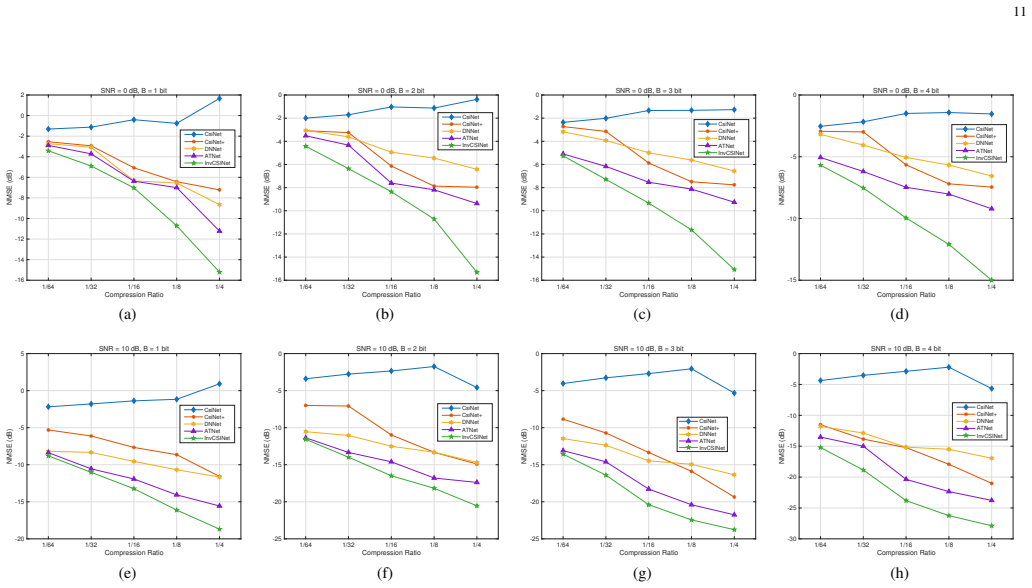
The central claim is that an invertible neural network (INN), a bijective map whose inverse is the decoder, can make CSI feedback information-preserving rather than information-losing. On the forward pass the network maps the channel matrix $H$ into a compressed feature $z$ and an auxiliary variable $r$ of dimension $N-M$; only $z$ is transmitted, and the decoder samples $r$ from a prior distribution, initially standard normal and later a learned Gaussian, before applying the inverse map to reconstruct the channel. Theorem 3 asserts that if the distribution-matching loss $L_r$ is driven to zero while the adaptive quantizer, bit-channel distortion module, and information-compensation module are trained jointly, then the recovered latent feature $\hat{z}$ at the base station equals the user-side compressed feature $z$, so the reconstructed channel distribution matches the true CSI distribution. The paper also reports simulations in an outdoor massive MIMO scenario where InvCSINet yields lower normalized mean square error than the autoencoder baselines across quantization bits and SNR levels, with parameters that grow slowly with the compression ratio.
Load-bearing premise
The scheme rests on the assumption that sampling the auxiliary variable $r$ at the decoder from a prior distribution can supply the information missing from the transmitted $z$, even though the particular $r$ produced by the encoder is discarded.
Editorial extensions
If this is right
- CSI feedback can be trained end-to-end with quantization and bit flips inside the computational graph, so the network adapts to the actual SNR and bit budget instead of treating impairments as post-hoc distortions.
- One shared parameter set serves as both encoder and decoder, so stored model size grows slowly with the compression dimension rather than doubling with separate encoder and decoder networks.
- In the zero-loss regime, reconstructed CSI is distributionally equivalent to true CSI, which would make statistical designs trained on true channel distributions see the same distribution at the decoder output.
- The reported gains over the four autoencoder baselines at 0 dB and 10 dB SNR with 1 to 4 quantization bits support the paper's claim that jointly modeling quantization and bit-channel errors is what improves reconstruction.
Reading between the lines
- An editorial reading: the zero-loss theorems guarantee distributional fidelity, not sample-wise recovery; a single decoded channel is one draw from the correct marginal, not necessarily the particular channel that was sent, because $r$ is sampled independently at the decoder.
- A test the paper does not run: for a fixed transmitted $z$, repeated decoding with fresh $r$ draws should have small reconstruction variance; if it does not, much of the reported NMSE improvement could come from the learned compensation layer rather than from sample-specific information.
- Because the bit-channel distortion module is just a transition-probability matrix, the same differentiable pipeline should extend to fading channels and higher-order modulation by substituting a different matrix, a step the paper does not demonstrate.
- If the scheme works as claimed, the combination of shared encoder-decoder parameters and distributional fidelity could be carried over to other limited-feedback tasks, such as precoder or channel-covariance feedback.
Editorial analysis
A structured set of objections, weighed in public.
Referee Report
Summary. The paper presents InvCSINet, an invertible-neural-network (INN) based framework for CSI feedback in FDD massive MIMO systems. The proposed method maps a high-dimensional CSI H to a compressed feature z and an auxiliary feature r via a bijective network, transmits only z, and at the base station samples r from a prior (or learned) distribution before applying the inverse network to reconstruct H. The paper claims that this design ensures 'information-preserving compression and reconstruction,' integrates differentiable quantization, channel-error, and information-compensation modules for end-to-end training, and proves (Theorems 2 and 3) that zero distribution-matching loss yields distributional fidelity of the reconstructed CSI. Simulations on DeepMIMO show NMSE improvements over several baselines across compression ratios, SNRs, and quantization bits.
Significance. If the information-preserving claim and the theorems were valid, the paper would make a strong contribution to learning-based CSI feedback, particularly for joint compression, quantization, and channel-error mitigation with shared encoder-decoder parameters. The empirical results suggest the architecture may be a competitive lossy CSI compression scheme. However, the core theoretical claim is unsupported: the decoder does not receive the true auxiliary variable r, so the invertibility of the INN is not actually exploited for sample-wise reconstruction, and the theorems only establish a distributional (not sample-wise) property, with proofs that are invalid. The paper's central selling point—'information-preserving' feedback—is therefore not substantiated.
major comments (5)
- [Section III-A, Eqs. (2)-(3)] The invertibility guarantee H = g(f(H)) requires the same auxiliary variable r that the encoder produced, but the decoder samples r from pR(r) (later from a learned υR(r)) because only z is transmitted. For a fixed H*, the encoder outputs a deterministic pair (z*, r*), yet the decoder computes g(z*, r̃) with r̃ ≠ r* almost surely, so g(z*, r̃) ≠ H*. The manuscript acknowledges in Section III-A that r is discarded and unavailable at the decoder, but it does not acknowledge that this invalidates the use of the bijection for sample-wise reconstruction. The 'information-preserving' claim collapses under this mismatch.
- [Appendix A, Eq. (38)] The proof of Theorem 2 replaces the deterministic encoder output r = fr(H*) with a sample from pR. For a single input H*, the conditional output distribution is q*(z,r) = δ(z − fz(H*))δ(r − fr(H*)), not δ(z − fz(H*))pR(r). The zero-MMD condition constrains the dataset-level marginal q(z,r) = p(z)pR(r), but it does not imply that the per-sample distribution factorizes in the manner written. Therefore Eq. (38) is invalid, and Theorem 2 is not proven.
- [Appendix B, Eqs. (42)-(44)] The proof of Theorem 3 is circular. Equation (42) asserts δ(ẑ − fz(H*)) = p(ẑ), which can hold only if p(ẑ) is degenerate at fz(H*), i.e., if the reconstruction chain (quantization, channel, LAN) is already identity—exactly the conclusion the theorem aims to establish. The subsequent equality (44) is therefore an assumption, not a consequence of the distributional matching. The notation also conflates the forward output z and the reconstructed latent ẑ. Theorem 3 is unproven.
- [Section V-B] The manuscript concedes that the MMD loss does not converge exactly to zero during training ('it is hard for the MMD metric to converge exactly to zero during training'), so the conditions of Theorems 2 and 3 are not met in the experiments. The theoretical guarantees cannot be invoked for the reported results, and the empirical NMSE gains should be interpreted only as the performance of a learned lossy compressor.
- [Abstract and Section I-B] The claim of 'information-preserving compression and reconstruction' is not supported by the theoretical results. Even if Theorems 2 and 3 were correct, they would only establish that the marginal distribution of reconstructed CSI matches the true distribution, which is a distributional property and does not imply that a specific CSI sample H can be recovered. The paper uses 'information preservation' in a way that conflates bijective invertibility (sample-wise recovery) with distributional matching; this is a load-bearing mischaracterization of the method's capability.
minor comments (5)
- [Section III-C, Eq. (8)] The notation p(z) in Eq. (8) is used for the marginal of the forward output, while Eq. (33) uses p(ẑ) for the marginal of the reconstructed latent; these should be clearly distinguished to avoid confusion in the MMD definitions.
- [Table II] The parameter comparison does not consistently show InvCSINet as the smallest model; at compression ratios 1/64 and 1/32, CsiNet has fewer parameters than InvCSINet. The 'lightweight architecture' claim should be qualified to specific regimes.
- [Section IV-B, Eq. (19)] There is a typographical issue in the summation index: the learnable parameter aq,i is defined with the same index q as the summation, but the text later refers to aQ−1,i; the index notation should be made consistent.
- [Section IV-C3] The heading 'Gumble-Softmax Sampling' contains a typo (should be 'Gumbel-Softmax'). In addition, the derivation of the transition probability matrix in Eq. (28) is specific to BPSK in AWGN; the claim that the model extends to other schemes should be supported by at least a brief description of how the TPM is generalized.
- [Lemma 1] The title 'Ditribution Preservation of INN' has a typo; it should read 'Distribution Preservation of INN'.
Circularity Check
Theorem 3 proves information preservation by assuming it: Eq. (42) equates the aggregate marginal p(\hat z) with a per-sample delta, so '\hat z equivalent to z' is the premise, not the conclusion.
-
self definitional
[Section IV-E, Theorem 3; Appendix B, Eqs. (42)-(44)]
"Connecting with (39), we have δ (ˆz − fz(H⋆)) = p(ˆz). (42) ... From (42) and (43), the following equality between z⋆ and ˆz⋆ can be achieved: ˆz⋆ = Ψ (Ω (ΛDAQ (fz(H⋆)) , ¯V)) = fz(H⋆). (44)"
The loss Lr = MMD2(q(z,r), p(ˆz)υR(r)) = 0 only equates distributions; at most it forces the marginal distribution of ˆz to equal that of z. It cannot force the deterministic pipeline ˆz = Ψ(Ω(Λ(z))) to be the identity on samples. Equation (42) writes δ(ˆz − fz(H⋆)) = p(ˆz), replacing the aggregate marginal density p(ˆz) with a delta at the transmitted feature of a single H⋆. That per-sample equality is exactly the conclusion 'ˆz becomes equivalent to z' that Theorem 3 claims to prove. Equation (44) then outputs fz(H⋆) = ˆz⋆ as a derived result, but it was already assumed in writing (42). The information-preserving claim is therefore the premise of the proof, not a consequence of zero MMD loss.
-
other
[Section III-A, Eq. (3) and overall framework; Appendix A, Eq. (38)]
"only the compressed feature z is transmitted to the BS, while the auxiliary feature r is discarded and unavailable at the decoder. ... Backward: H = g(z, r; θ), with r ∼ pR(r) = N (r; 0, I)."
The inversion guarantee of the INN is for f(H) = [z, r]; the decoder however receives only z and draws a fresh r from pR. Equation (38) asserts q⋆(z, r) = δ(z − fz(H⋆))pR(r), thereby replacing the deterministic encoder output r = fr(H⋆) with an independent sample from the prior. For a fixed H⋆ the r-marginal is δ(r − fr(H⋆)), not pR(r); the equality holds only in aggregate over the dataset. Using it to justify H = g(z, r_sampled) as information-preserving assumes that the discarded information in r is recoverable from its prior, which is exactly the claim under test. The proof therefore assumes, rather than establishes, the conclusion that sample-wise reconstruction is preserved.
full rationale
The empirical architecture is evaluated against external baselines on DeepMIMO, so those performance comparisons are not circular. The theoretical layer, however, is: Theorem 3's conclusion that the recovered latent equals the transmitted latent is inserted into the proof as Eq. (42), where the aggregate marginal p(ˆz) is written as a per-sample delta at fz(H⋆). Zero MMD loss supplies only distributional equality, not pointwise equality; the pointwise equality is the 'information-preserving' claim itself. The same substitution occurs for r: Eq. (38) replaces the encoder's deterministic r with a fresh sample from pR, which is legitimate only for distributional fidelity, not sample-wise preservation. Hence the central abstract claim 'information-preserving compression and reconstruction' reduces, in the proof, to the assumption that the untransmitted auxiliary variable and the reconstructed latent carry the discarded information. The paper also concedes in Section V-B that the MMD loss does not converge to zero during training, so even the stated distributional condition is not met in practice.
Assumptions & free parameters
free parameters (5)
- Learnable auxiliary prior mean mu and variance sigma^2 =
Learned, not reported in the paper
- MMD trade-off parameter kappa =
0.1
- MMD kernel constant C =
1000
- Initial quantization range (zmin, zmax) =
(-2, 2)
- Soft quantization sharpness T, soft-mapping beta, Gumbel temperature tau =
Not specified
assumptions (5)
- standard math Lemma 1: A bijective function that transforms pX to pZ also transforms pZ back to pX via its inverse.
- domain assumption The MMD loss Lr can be driven to exactly zero.
- ad hoc to paper A decoder using z and an independently sampled r can reconstruct the original specific H sample-wise.
- domain assumption The auxiliary variable r follows a Gaussian prior (N(0,I) or a learned N(mu, sigma^2 I)).
- domain assumption The feedback channel is modeled as BPSK over AWGN with bit error probability Q(sqrt(gamma)).
invented entities (1)
-
Auxiliary variable r (dimension N-M)
Cite this review
Pith. "Pith review of Information-Preserving CSI Feedback: Invertible Networks with Endogenous Quantization and Channel Error Mitigation." pith.science (2026). https://pith.science/paper/7S36DWF5
@misc{pith2026250720283,
  author       = {Pith},
  title        = {Pith review of: Information-Preserving CSI Feedback: Invertible Networks with Endogenous Quantization and Channel Error Mitigation},
  year         = {2026},
  howpublished = {\url{https://pith.science/paper/7S36DWF5}},
  note         = {Machine review of arXiv:2507.20283}
}
read the original abstract
Deep learning has emerged as a promising solution for efficient channel state information (CSI) feedback in frequency division duplex (FDD) massive MIMO systems. Conventional deep learning-based methods typically rely on a deep autoencoder to compress the CSI, which leads to irreversible information loss and degrades reconstruction accuracy. This paper introduces InvCSINet, an information-preserving CSI feedback framework based on invertible neural networks (INNs). By leveraging the bijective nature of INNs, the model ensures information-preserving compression and reconstruction with shared model parameters. To address practical challenges such as quantization and channel-induced errors, we endogenously integrate an adaptive quantization module, a differentiable bit-channel distortion module and an information compensation module into the INN architecture. This design enables the network to learn and compensate the information loss during CSI compression, quantization, and noisy transmission, thereby preserving the CSI integrity throughout the feedback process. Simulation results validate the effectiveness of the proposed scheme, demonstrating superior CSI recovery performance and robustness to practical impairments with a lightweight architecture.
Figures


Figures from the paper (5 more)


Reference graph
Works this paper leans on
-
[1]
Noncooperative Cellular Wireless with Unlimited Numbers of Base Station Antennas,
T. L. Marzetta, “Noncooperative Cellular Wireless with Unlimited Numbers of Base Station Antennas,” IEEE Trans. Wireless Commun. , vol. 9, no. 11, pp. 3590–3600, 2010
work page 2010
-
[2]
Massive MIMO in the UL/DL of cellular networks: How many antennas do we need?
J. Hoydis, S. Ten Brink, and M. Debbah, “Massive MIMO in the UL/DL of cellular networks: How many antennas do we need?” IEEE J. Sel. Areas Commun., vol. 31, no. 2, pp. 160–171, 2013
work page 2013
-
[3]
Limited feedback channel estimation in massive MIMO with non- uniform directional dictionaries,
P. N. Alevizos, X. Fu, N. D. Sidiropoulos, Y . Yang, and A. Bletsas, “Limited feedback channel estimation in massive MIMO with non- uniform directional dictionaries,” IEEE Trans. Signal Process. , vol. 66, no. 19, pp. 5127–5141, 2018
work page 2018
-
[4]
An overview of limited feedback in wireless communication systems,
D. J. Love, R. W. Heath, V . K. Lau, D. Gesbert, B. D. Rao, and M. An- drews, “An overview of limited feedback in wireless communication systems,” IEEE J. Sel. Areas Commun. , vol. 26, no. 8, pp. 1341–1365, 2008
work page 2008
-
[5]
J. Kang and W. Choi, “Novel codebook design for channel state information quantization in MIMO rician fading channels with limited feedback,” IEEE Trans. Signal Process. , vol. 69, pp. 2858–2872, 2021
work page 2021
-
[6]
Downlink channel estimation in multiuser massive MIMO with hidden Markovian sparsity,
A. Liu, L. Lian, V . K. Lau, and X. Yuan, “Downlink channel estimation in multiuser massive MIMO with hidden Markovian sparsity,” IEEE Trans. Signal Process. , vol. 66, no. 18, pp. 4796–4810, 2018
work page 2018
-
[7]
Joint massive MIMO CSI estimation and feedback via randomized low-rank approximation,
Z. Wei, H. Liu, B. Li, and C. Zhao, “Joint massive MIMO CSI estimation and feedback via randomized low-rank approximation,” IEEE Trans. V eh. Technol., vol. 71, no. 7, pp. 7979–7984, 2022
work page 2022
-
[8]
K. Li, Y . Li, L. Cheng, Q. Shi, and Z.-Q. Luo, “Downlink channel covariance matrix reconstruction for FDD massive MIMO systems with limited feedback,” IEEE Trans. Signal Process. , vol. 72, pp. 1032–1048, 2024
work page 2024
Show all 36 references
-
[9]
Overview of deep learning- based CSI feedback in massive MIMO systems,
J. Guo, C.-K. Wen, S. Jin, and G. Y . Li, “Overview of deep learning- based CSI feedback in massive MIMO systems,” IEEE Trans. Commun., vol. 70, no. 12, pp. 8017–8045, 2022
2022
-
[10]
Deep learning for massive MIMO CSI feedback,
C.-K. Wen, W.-T. Shih, and S. Jin, “Deep learning for massive MIMO CSI feedback,” IEEE Wireless Commun. Lett., vol. 7, no. 5, pp. 748–751, 2018
2018
-
[11]
CLNet: Complex Input Lightweight Neural Network Designed for Massive MIMO CSI Feedback,
S. Ji and M. Li, “CLNet: Complex Input Lightweight Neural Network Designed for Massive MIMO CSI Feedback,” IEEE Wireless Commu- nications Letters , vol. 10, no. 10, pp. 2318–2322, 2021
2021
-
[12]
A Novel Quantization Method for Deep Learning-Based Massive MIMO CSI Feedback,
T. Chen, J. Guo, S. Jin, C. Wen, and G. Y . Li, “A Novel Quantization Method for Deep Learning-Based Massive MIMO CSI Feedback,” in Proc. IEEE Glob. Conf. Signal Inf. Process. (GlobalSIP) , 2019, pp. 1– 5
2019
-
[13]
Deep joint source-channel coding for CSI feedback: An end-to-end approach,
J. Xu, B. Ai, N. Wang, and W. Chen, “Deep joint source-channel coding for CSI feedback: An end-to-end approach,” IEEE J. Sel. Areas Commun., vol. 41, no. 1, pp. 260–273, 2022
2022
-
[14]
Multi-resolution CSI feedback with deep learning in massive MIMO system,
Z. Lu, J. Wang, and J. Song, “Multi-resolution CSI feedback with deep learning in massive MIMO system,” in Proc. IEEE Int. Conf. Commun. (ICC), 2020, pp. 1–6
2020
-
[15]
CSI- StripeFormer: Exploiting stripe features for CSI compression in massive MIMO system,
Q. Hu, H. Kang, H. Chen, Q. Huang, Q. Zhang, and M. Cheng, “CSI- StripeFormer: Exploiting stripe features for CSI compression in massive MIMO system,” in Proc. IEEE Conf. Comput. Commun. (INFOCOM) , 2023, pp. 1–10
2023
-
[16]
Bayesian Hierarchical Sparse Autoencoder for Massive MIMO CSI Feedback,
H. Guo and V . K. Lau, “Bayesian Hierarchical Sparse Autoencoder for Massive MIMO CSI Feedback,” IEEE Trans. Signal Process. , vol. 72, pp. 3213–3227, 2024
2024
-
[17]
Deep learning-based denoise network for CSI feedback in FDD massive MIMO systems,
H. Ye, F. Gao, J. Qian, H. Wang, and G. Y . Li, “Deep learning-based denoise network for CSI feedback in FDD massive MIMO systems,” IEEE Commun. Lett. , vol. 24, no. 8, pp. 1742–1746, 2020
2020
-
[18]
Deep learning-based bitstream error correction for CSI feedback,
H. Chang, X. Liang, H. Li, J. Shen, X. Gu, and L. Zhang, “Deep learning-based bitstream error correction for CSI feedback,” IEEE Wireless Commun. Lett. , vol. 10, no. 12, pp. 2828–2832, 2021
2021
-
[19]
Deep autoencoder-based massive MIMO CSI feedback with quantization and entropy coding,
S. Ravula and S. Jain, “Deep autoencoder-based massive MIMO CSI feedback with quantization and entropy coding,” in Proc. IEEE Global Commun. Conf. (GLOBECOM) , 2021, pp. 1–6
2021
-
[20]
Deep learning-based CSI feedback approach for time-varying massive MIMO channels,
T. Wang, C.-K. Wen, S. Jin, and G. Y . Li, “Deep learning-based CSI feedback approach for time-varying massive MIMO channels,” IEEE Wireless Commun. Lett. , vol. 8, no. 2, pp. 416–419, 2018
2018
-
[21]
Binarized aggregated network with quantization: Flexible deep learning deployment for CSI feedback in massive MIMO systems,
Z. Lu, X. Zhang, H. He, J. Wang, and J. Song, “Binarized aggregated network with quantization: Flexible deep learning deployment for CSI feedback in massive MIMO systems,” IEEE Trans. Wireless Commun. , vol. 21, no. 7, pp. 5514–5525, 2022
2022
-
[22]
Convolutional neural network- based multiple-rate compressive sensing for massive MIMO CSI feed- back: Design, simulation, and analysis,
J. Guo, C.-K. Wen, S. Jin, and G. Y . Li, “Convolutional neural network- based multiple-rate compressive sensing for massive MIMO CSI feed- back: Design, simulation, and analysis,” IEEE Trans. Wireless Commun., vol. 19, no. 4, pp. 2827–2840, 2020
2020
-
[23]
Changeable rate and novel quantization for CSI feedback based on deep learning,
X. Liang, H. Chang, H. Li, X. Gu, and L. Zhang, “Changeable rate and novel quantization for CSI feedback based on deep learning,” IEEE Trans. Wireless Commun. , vol. 21, no. 12, pp. 10 100–10 114, 2022
2022
-
[24]
Quantization Adaptor for Bit-Level Deep Learning-Based Massive MIMO CSI Feedback,
X. Zhang, Z. Lu, R. Zeng, and J. Wang, “Quantization Adaptor for Bit-Level Deep Learning-Based Massive MIMO CSI Feedback,” IEEE Trans. V eh. Technol., vol. 73, no. 4, pp. 5443–5453, 2023
2023
-
[25]
An efficient deep learning framework for low rate massive MIMO CSI reporting,
Z. Liu, L. Zhang, and Z. Ding, “An efficient deep learning framework for low rate massive MIMO CSI reporting,” IEEE Trans. Commun., vol. 68, no. 8, pp. 4761–4772, 2020
2020
-
[26]
Information Bottleneck Based Joint Feedback and Channel Learning in FDD Massive MIMO Systems,
J. Cao and L. Lian, “Information Bottleneck Based Joint Feedback and Channel Learning in FDD Massive MIMO Systems,” in Proc. IEEE Global Commun. Conf. , 2022, pp. 1442–1447
2022
-
[27]
Adaptive CSI Feedback with Hidden Semantic Information Transfer,
J. Cao, L. Lian, Y . Mao, and B. Clerckx, “Adaptive CSI Feedback with Hidden Semantic Information Transfer,” in Proc. IEEE Int. Conf. Acoust., Speech Signal Process. (ICASSP) , 2023, pp. 1–5
2023
-
[28]
Analyz- ing inverse problems with invertible neural networks,
L. Ardizzone, J. Kruse, S. Wirkert, D. Rahner, E. W. Pellegrini, R. S. Klessen, L. Maier-Hein, C. Rother, and U. Köthe, “Analyz- ing inverse problems with invertible neural networks,” arXiv preprint arXiv:1808.04730, 2018
2018 arXiv
-
[29]
Density estimation using real nvp,
L. Dinh, J. Sohl-Dickstein, and S. Bengio, “Density estimation using real nvp,” arXiv preprint arXiv:1605.08803 , 2016
2016 arXiv
-
[30]
Glow: Generative Flow with Invertible 1x1 Convolutions,
D. P. Kingma and P. Dhariwal, “Glow: Generative Flow with Invertible 1x1 Convolutions,” in Proc. Adv. Neural Inf. Process. Syst. (NeurIPS) , vol. 31, 2018, pp. 10 236–10 245
2018
-
[31]
A Kernel Two-Sample Test,
A. Gretton, K. M. Borgwardt, M. J. Rasch, B. Schölkopf, and A. J. Smola, “A Kernel Two-Sample Test,” J. Mach. Learn. Res. , vol. 13, pp. 723–773, 2012
2012
-
[32]
Wasserstein auto-encoders,
I. Tolstikhin, O. Bousquet, S. Gelly, and B. Schoelkopf, “Wasserstein auto-encoders,” arXiv preprint arXiv:1711.01558 , 2017
2017 arXiv
-
[33]
Hashnet: Deep learning to hash by continuation,
Z. Cao, M. Long, J. Wang, and P. S. Yu, “Hashnet: Deep learning to hash by continuation,” in Proc. IEEE Int. Conf. Comput. Vis. (ICCV) , 2017, pp. 5608–5617
2017
-
[34]
Categorical reparameterization with gumbel-softmax,
E. Jang, S. Gu, and B. Poole, “Categorical reparameterization with gumbel-softmax,” arXiv preprint arXiv:1611.01144 , 2016
2016 arXiv
-
[35]
DeepMIMO: A generic deep learning dataset for millimeter wave and massive MIMO applications,
A. Alkhateeb, “DeepMIMO: A generic deep learning dataset for millimeter wave and massive MIMO applications,” arXiv preprint arXiv:1902.06435, 2019
1902 arXiv
-
[36]
Adam: A Method for Stochastic Optimization,
D. Kingma and J. Ba, “Adam: A Method for Stochastic Optimization,” in Proc. Int. Conf. Learn. Represent. (ICLR) , San Diega, CA, USA, 2015
2015
Reviewed August 6, 2026 · model on record in the stance chip above.
Discussion (0). Sign in to comment.