REVIEW 3 major objections 4 minor 48 references
Regression Analysis of Reciprocity in Directed Networks
T0 review · 3 major / 4 minor · reviewed 2026-08-06 · deepseek-v4-flash
Pith's one-line read This paper introduces the R²-Model, which regresses reciprocity on dyad covariates while removing node heterogeneity by conditioning on four-node subgraphs, and proves the resulting estimator is minimax rate-optimal.
desk verdict Solid, important extension of tetrad conditioning to directed networks with reciprocity; watch the bounded-heterogeneity assumption before you trust the advertised scope. read the letter →
The pith
A machine-rendered reading of the paper's core claim, the machinery that carries it, and where it could break.
The reading
What carries the argument
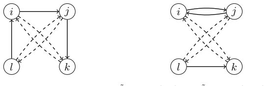
The load-bearing object is the tetrad statistic $S_{ijkl}\in\{0,+1,-1\}$: three directed configurations on four nodes that are edge-rewirings of one another and therefore share the same in- and out-degree sequence. Conditioning on $S_{ijkl}\in\{0,\pm1\}$ cancels the density parameter and all $2n$ node heterogeneity terms, leaving a three-outcome likelihood with probabilities $1/(1+r)$, $f/(1+r)$, $g/(1+r)$ that depend only on $\rho_n$ and $\gamma$—this is the mechanism that isolates the reciprocity effects. The convergence rates are set by the sparsity indices $a$ and $b$: the three tetrad events have probabilities of order $n^{-4a}$ and $n^{-4a+2b}$, so the score and Hessian need different normalizations in different regimes, and asymptotic normality is proved by viewing the score as a $U$-statistic and showing its Hájek projection onto dyads dominates the variance.
What would settle it
Simulate the model with a fixed sparsity regime ($a,b$), node sizes growing from $n=50$ to $n=200$, and $\alpha_i,\beta_i$ drawn so that $\max_i|\alpha_i|$ grows with $n$ (e.g., Pareto tails), rather than bounded as Assumption 2 requires; compare the empirical frequencies of the three tetrad types against $n^{-4a}$ and $n^{-4a+2b}$, and check whether the Theorem 3 confidence intervals for $\rho_n$ and $\gamma$ keep their nominal 95% coverage. A widening coverage gap as $\max_i|\alpha_i|$ grows would show where the minimax claim breaks.
Extended reading notes
Core claim
The paper's central claim is that the reciprocity parameters can be estimated at the statistically optimal rate despite the presence of $2n$ nuisance parameters and sparsity. Explicitly, with sparsity indices $a,b$ defined by $\mu_n = -a\log n$ and $\rho_n = b\log n$, the tetrad-based conditional likelihood estimator satisfies $\sqrt{n^{2-2a+\min\{a,b\}}}(\hat{\rho}_n - \rho_{n0}) \to N(0,\sigma_\rho^2)$ and $\sqrt{n^{2-2a+b}}(\hat{\gamma}-\gamma_0) \to N(0,\Sigma_\gamma)$, and Theorem 4 proves that no estimator over the parameter class can achieve mean squared error smaller than $n^{-2+2a-\min\{a,b\}}$ for $\rho_n$ or $n^{-2+2a-b}$ for $\gamma$. The same construction gives a feasible inference procedure, Theorem 3, which does not require knowing $a$ or $b$.
Load-bearing premise
The theory assumes every node's sender and receiver effects are bounded by a constant independent of $n$; if a network has hubs or extremely inactive nodes, the tetrad event probabilities and all rates built on them no longer hold.
Editorial extensions
If this is right
- Practitioners can test whether reciprocity varies with covariates using confidence intervals computed from Theorem 3 without knowing the sparsity parameters $a$ and $b$.
- In the classical $p_1$ model (no covariates), the estimator reduces to a closed-form log-ratio of tetrad counts, providing a simple method-of-moments-style estimator of baseline reciprocity.
- When reciprocity is strong ($b > a$), the covariate slopes are estimated at a strictly faster rate than the baseline reciprocity, because comparisons between the two $\pm1$ tetrad configurations carry information about $\gamma$ only.
- The minimax lower bounds apply to all estimators, not just conditional likelihood ones, so no alternative estimator can beat the proposed rates in the moderate-heterogeneity regime.
Reading between the lines
- The same tetrad-conditioning design should transfer to models with edgewise homophily covariates, because the sufficiency lemma only requires configurations sharing the same degree sequence; a direct implementation would give inference on the homophily slope without node-effect estimation.
- A simulation with heavy-tailed $\alpha_i,\beta_i$ (for example, Pareto-distributed) would likely show tetrad frequencies and coverage degrading, marking the empirical boundary of Assumption 2; this is a concrete testable extension the paper does not run.
- Although the theory is stated for a single network snapshot, the log-odds structure suggests the estimator could be adapted to panel or multi-layer directed networks by treating each layer's degree sequences as the conditioning statistic—an extension the authors do not pursue.
- The closed-form estimator of Proposition 1 (a log ratio of tetrad counts) hints at an interpretation of the R²-Model as comparing two oriented 4-cycles; this connection suggests the methodology could be exported to any dyadic outcome model where a sufficient statistic can be frozen by degree-preserving rewirings.
Signed reviews
Editorial analysis
A structured set of objections, weighed in public.
Referee Report
Summary. The paper introduces the R²-Model, a generalized p1 model for directed networks that incorporates reciprocity through a baseline parameter ρ_n and a covariate vector γ, while allowing node-specific sender and receiver heterogeneity. To avoid estimating 2n+2+q parameters, the authors propose a conditional likelihood estimator based on tetrad configurations that conditions out the degree sequence and isolates (ρ_n, γ). They prove consistency, asymptotic normality, and minimax rate optimality under sparsity assumptions, and support the results with simulations and two empirical applications. The proof strategy relies on U-statistic projections and a case-by-case analysis of tetrad dependence, with complete proofs in the supplementary material.
Significance. If the results hold, this is a useful and nontrivial extension of Graham's tetrad-based conditional likelihood approach to directed networks with reciprocity and covariates. The paper provides machine-checkable auxiliary material in the form of detailed proofs, and it gives a constructive proof of minimax optimality via Le Cam's two-point method, which is a strong selling point. The closed-form estimator for the p1 submodel and the real-data applications increase the paper's practical appeal. However, the theoretical guarantees are established only under a bounded-heterogeneity assumption, which is narrower than the paper's advertised 'unrestricted' heterogeneity, and the numerical studies lack a description of how the computationally heavy tetrad enumeration was performed.
major comments (3)
- [Section 1, p.2; Section 2.2, Assumption 2] The paper repeatedly claims to allow 'unrestricted node-level heterogeneity' (Section 1) and the abstract states the model 'accommodates both network sparsity and node heterogeneity,' but Assumption 2 requires max_i{|α_i|,|β_i|} ≤ C for a constant independent of n. This uniform boundedness is load-bearing: Lemma 1's event probabilities, Lemma 2's derivative bounds, Proposition 2's covariance orders, and the rates in Theorems 2 and 3 all use it. If max_i|α_i| were to grow with n, say as C log n, then the probabilities P(S_ijkl=0) ∼ n^{-4a} and P(S_ijkl=±1) ∼ n^{-4a+2b} would fail, and the U-statistic variance decomposition would collapse. The authors should either weaken the stated claims to 'moderate degree heterogeneity' or extend the theory to slowly growing heterogeneity with explicit rate conditions.
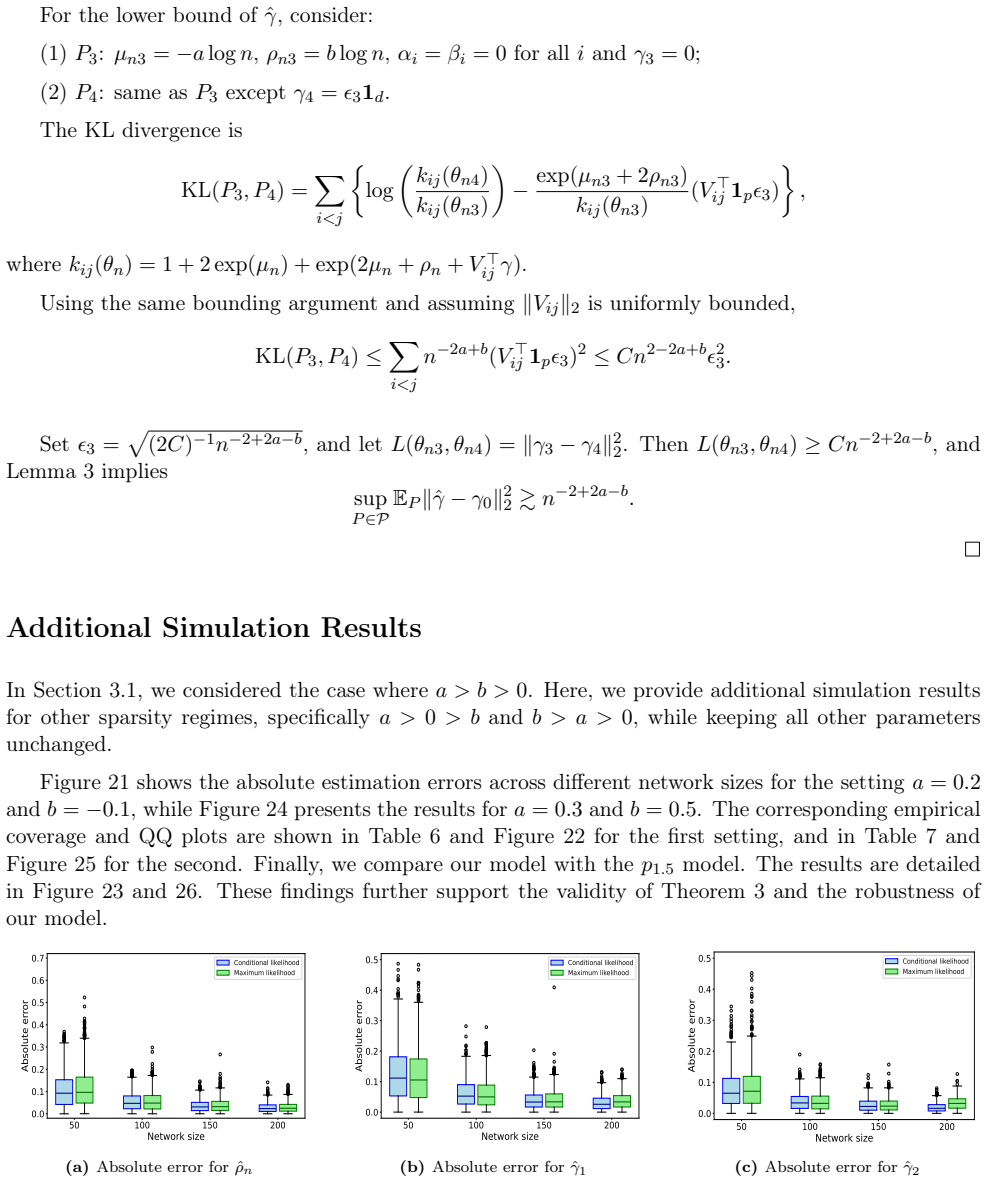
- [Section 3.1, simulations] The numerical study reports 1000 replications for n = 50, 100, 150, 200 without explaining how the estimator L_n, which sums over all C(n,4) tetrads, was computed. For n=200 there are approximately 6.5×10^7 tetrads per replication, making the reported 1000 replications (about 6.5×10^10 tetrad evaluations per setting) computationally infeasible with the described full enumeration. If a random subsample of tetrads or another approximation was used, that estimator is not covered by Theorems 1-3, and the finite-sample claims and confidence-interval coverages need to be justified for the implemented procedure. The paper should state the exact algorithm and, if subsampling is used, provide a corresponding theoretical statement.
- [Supplementary, proof of Theorem 2, Case C] In the proof of Theorem 2, Case C, the text states 'ˆρ − ρ0 = ... = OP(1)' after having shown n^{4a}Ψ_{n,ρ}(ϑ0) = OP(n^{(-2+a)/2}) and that the scaled Hessian is Θ(1). This implies the difference should be OP(n^{-1+a/2}), not OP(1). This is a typographical error, but it obscures the convergence rate and should be corrected in the supplementary material.
minor comments (4)
- [Section 2.2, Theorem 3] Theorem 3 uses the normalization 'n · (ˆρ_n − ρ_n0) / sqrt(Σ̂_1,1)', which is correct because the variance estimator Σ̂ automatically scales as n^{2a-b} (or n^a in the b>a case), but the statement would be clearer with explicit parentheses, e.g., 'n(ˆρ_n − ρ_{n0})'. The stray 'q' artifacts in the displayed formulas should also be cleaned.
- [Supplementary, proof of Proposition 1] The proof of Proposition 1 derives ˆρ_n = (1/2) log( Σ I(S=1) / Σ I(S=0) ), while the proposition states the numerator as Σ I(S=±1). The numerator should be I(S=±1) to match the first-order condition; the current text is inconsistent.
- [Section 1, model definition] The covariate V_ij is defined for i<j in Assumption 1, but the model formulas use V_il and V_jk for the S=-1 configuration. Since these expressions are only well-defined if V_ij = V_ji, the paper should state explicitly that dyadic covariates are symmetric.
- [Supplementary, Proposition 2 statement] Proposition 2 states Var(τ_n ⊙ τ_n ⊙ Ψ_n(ϑ)) = o(1), but the proof analyzes Var(τ_n ⊙ Ψ_n(ϑ)). The extra 'τ_n ⊙' appears to be a typo and should be removed.
Circularity Check
No circularity: the estimator and minimax rates are derived from the model, with no fitted parameter renamed as a prediction.
full rationale
The derivation chain is self-contained. Lemma 1 computes the tetrad conditional probabilities directly from the model in (2), eliminating the nuisance parameters and leaving a likelihood in (rho, gamma). The score bounds in Lemma 2 and the variance decomposition in Proposition 2 are proved from the model's event probabilities P(S_ijkl = 0) ~ n^{-4a} and P(S_ijkl = +/-1) ~ n^{-4a+2b}, so the rates in Theorems 1-3 are consequences of the model rather than assumptions. The minimax lower bound in Theorem 4 uses Le Cam's two-point method over the parameter class Theta_n, with explicit perturbations chosen so that the KL divergence is bounded; the matching upper bounds come from Theorem 2, so the optimality claim does not reduce to a fitted constant or to a self-citation. The self-citations to Feng and Leng (2025), including the phrase 'effective sample size', are contextual: the proofs cite no theorem from that paper, and the scaling is derived in Lemmas 2 and Proposition 2. The bounded-heterogeneity restriction in Assumption 2 is a stated scope limitation rather than a circular step; it narrows the regime but does not define the conclusions in terms of the inputs.
Assumptions & free parameters
free parameters (2)
- sparsity exponent a =
not fitted; assumed (simulations use a=0.2 or 0.3)
- reciprocity exponent b =
not fitted; assumed (simulations use b=0.1, -0.1, or 0.5)
assumptions (5)
- domain assumption Dyads (A_ij, A_ji) are mutually independent conditional on covariates and node-specific parameters alpha and beta.
- domain assumption Assumption 1: covariates V_ij are centered, i.i.d., and uniformly bounded; true parameter lies in the interior of a compact set.
- domain assumption Assumption 2: max_i {|alpha_i|, |beta_i|} <= C for a constant C independent of n.
- domain assumption Assumption 3: 0 < a < 1 and 0 < 2a - b < 2; Assumption 5: a < 2/3 for asymptotic normality.
- standard math Assumptions 4 and 6: the scaled score and Hessian converge to non-random limits, and the limiting information matrix is positive definite.
Cite this review
Pith. "Pith review of Regression Analysis of Reciprocity in Directed Networks." pith.science (2026). https://pith.science/paper/ORNZMUCH
@misc{pith2026250721469,
  author       = {Pith},
  title        = {Pith review of: Regression Analysis of Reciprocity in Directed Networks},
  year         = {2026},
  howpublished = {\url{https://pith.science/paper/ORNZMUCH}},
  note         = {Machine review of arXiv:2507.21469}
}
abstract
Reciprocity--the tendency of individuals to form mutual ties--is a fundamental structural feature of many directed networks. Despite its ubiquity, reciprocity remains insufficiently integrated into statistical network models, particularly in relation to covariate information. In this paper, we introduce the $R^{2}$-Model, a novel and flexible framework that explicitly models reciprocity while incorporating covariate effects. Built upon a generalized $p_1$ model, our framework accommodates both network sparsity and node heterogeneity, offering the most comprehensive parametrization of reciprocity to date--capturing not only its baseline level but also how it systematically varies with observed covariates. To address the challenges posed by high dimensionality and nuisance parameters, we develop a conditional likelihood estimator that isolates and consistently estimates the reciprocity effects. We establish its theoretical guarantees, including consistency, asymptotic normality, and minimax optimality under broad sparsity regimes. Extensive simulations and real-world applications demonstrate the $R^{2}$-Model's flexibility, interpretability, and strong finite-sample performance, highlighting its practical utility for uncovering covariate-driven patterns of reciprocity in directed networks.
Figures


Figures from the paper (23 more)




Reference graph
Works this paper leans on
-
[1]
Anderson, J. E. (2011). The gravity model. Annual Review of Economics , 3(1):133--160
work page 2011
-
[2]
Barab \'a si, A.-L. and Albert, R. (1999). Emergence of scaling in random networks. Science , 286(5439):509--512
work page 1999
-
[3]
Barndorff-Nielsen, O. (1983). On a formula for the distribution of the maximum likelihood estimator. Biometrika , 70(2):343--365
work page 1983
-
[4]
Barndorff-Nielsen, O. E. and McCullagh, P. (1993). A note on the relation between modified profile likelihood and the cox-reid adjusted profile likelihood. Biometrika , 80(2):321--328
work page 1993
-
[5]
Bartlett, M. S. (1937). Properties of sufficiency and statistical tests. Proceedings of the Royal Society of London. Series A-Mathematical and Physical Sciences , 160(901):268--282
work page 1937
-
[6]
D., Yao, Q., and Yi, F
Chang, J., Hu, Q., Kolaczyk, E. D., Yao, Q., and Yi, F. (2024). Edge differentially private estimation in the -model via jittering and method of moments. The Annals of Statistics , 52(2):708--728
2024
-
[7]
Charbonneau, K. B. (2017). Multiple fixed effects in binary response panel data models. The Econometrics Journal , 20(3):S1--S13
work page 2017
-
[8]
Chen, M., Kato, K., and Leng, C. (2021). Analysis of networks via the sparse -model. Journal of the Royal Statistical Society Series B: Statistical Methodology , 83(5):887--910
work page 2021
Show all 48 references
-
[9]
and Kato, K
Chen, X. and Kato, K. (2019). Randomized incomplete u -statistics in high dimensions. The Annals of Statistics , 47(6):3127--3156
2019
-
[10]
Cox, D. R. and Reid, N. (1987). Parameter orthogonality and approximate conditional inference. Journal of the Royal Statistical Society: Series B (Methodological) , 49(1):1--18
1987
-
[11]
Dorogovtsev, S. N. and Mendes, J. F. F. (2003). Evolution of Networks: From Biological Nets to the Internet and WWW . Oxford University Press
2003
-
[12]
Dzemski, A. (2019). An empirical model of dyadic link formation in a network with unobserved heterogeneity. Review of Economics and Statistics , 101(5):763--776
2019
-
[13]
and Leng, C
Feng, R. and Leng, C. (2025). Modelling directed networks with reciprocity. Biometrika , 112(2):asaf035
2025
-
[14]
and Weidner, M
Fern \'a ndez-Val, I. and Weidner, M. (2016). Individual and time effects in nonlinear panel models with large n, t. Journal of Econometrics , 192(1):291--312
2016
-
[15]
Fienberg, S. E. (2012). A brief history of statistical models for network analysis and open challenges. Journal of Computational and Graphical Statistics , 21(4):825--839
2012
-
[16]
and Loffredo, M
Garlaschelli, D. and Loffredo, M. I. (2004). Patterns of link reciprocity in directed networks. Physical Review Letters , 93(26):268701
2004
-
[17]
Graham, B. S. (2017). An econometric model of network formation with degree heterogeneity. Econometrica , 85(4):1033--1063
2017
-
[18]
Handcock, M. S. and Gile, K. J. (2010). Modeling social networks from sampled data. The Annals of Applied Statistics , 4(1):5--25
2010
-
[19]
Holland, P. W. and Leinhardt, S. (1981). An exponential family of probability distributions for directed graphs. Journal of the American Statistical Association , 76(373):33--50
1981
-
[20]
Horn, R. A. and Johnson, C. R. (2012). Matrix analysis . Cambridge university press
2012
-
[21]
Hunter, D. R. and Handcock, M. S. (2006). Inference in curved exponential family models for networks. Journal of Computational and Graphical Statistics , 15(3):565--583
2006
-
[22]
Jackson, M. O. (2008). Social and Economic Networks . Princeton University Press
2008
-
[23]
and Jin, J
Ji, P. and Jin, J. (2016). Coauthorship and citation networks for statisticians. The Annals of Applied Statistics , 10(4):1779--1812
2016
-
[24]
Jiang, B., Zhang, Z.-L., and Towsley, D. (2015). Reciprocity in social networks with capacity constraints. In Proceedings of the 21th ACM SIGKDD International Conference on Knowledge Discovery and Data Mining , pages 457--466
2015
-
[25]
T., Luo, S., and Ma, Y
Jin, J., Ke, Z. T., Luo, S., and Ma, Y. (2025). Optimal network pairwise comparison. Journal of the American Statistical Association , 120(550):1048--1062
2025
-
[26]
Jochmans, K. (2018). Semiparametric analysis of network formation. Journal of Business & Economic Statistics , 36(4):705--713
2018
-
[27]
Kolaczyk, E. D. (2009). Statistical Analysis of Network Data: Methods and Models . Springer
2009
-
[28]
Krivitsky, P. N. and Kolaczyk, E. D. (2015). On the question of effective sample size in network modeling: an asymptotic inquiry. Statistical Science , 30(2):184--198
2015
-
[29]
Lazega, E. (2001). The Collegial Phenomenon: The Social Mechanisms of Cooperation Among Peers in a Corporate Law Partnership . Oxford University Press
2001
-
[30]
Lou, T., Tang, J., Hopcroft, J., Fang, Z., and Ding, X. (2013). Learning to predict reciprocity and triadic closure in social networks. ACM Transactions on Knowledge Discovery from Data (TKDD) , 7(2):1--25
2013
-
[31]
Ma, Z., Ma, Z., and Yuan, H. (2020). Universal latent space model fitting for large networks with edge covariates. Journal of Machine Learning Research , 21(4):1--67
2020
-
[32]
Newman, M. (2018). Networks . Oxford university press
2018
-
[33]
E., Forrest, S., and Balthrop, J
Newman, M. E., Forrest, S., and Balthrop, J. (2002). Email networks and the spread of computer viruses. Physical Review E , 66(3):035101
2002
-
[34]
Petrovic, S., Rinaldo, A., and Fienberg, S. E. (2010). Algebraic statistics for a directed random graph model with reciprocation. Contemporary Mathematics , 516:261–283
2010
-
[35]
Rinaldo, A., Petrovi \'c , S., and Fienberg, S. (2010). On the existence of the MLE for a directed random graph network model with reciprocation. arXiv , 2010
2010
-
[36]
Shao, M., Xia, D., and Zhang, Y. (2025). U-statistic reduction: Higher-order accurate risk control and statistical-computational trade-off. Journal of the American Statistical Association
2025
-
[37]
Shao, M., Zhang, Y., Wang, Q., Zhang, Y., Luo, J., and Yan, T. (2021). L-2 regularized maximum likelihood for -model in large and sparse networks. arXiv preprint arXiv:2110.11856
2021 arXiv
-
[38]
Silva, J. M. C. S. and Tenreyro, S. (2006). The log of gravity. The Review of Economics and Statistics , 88(4):641--658
2006
-
[39]
Stein, S., Feng, R., and Leng, C. (2025). A sparse beta regression model for network analysis. Journal of the American Statistical Association , 120(550):1281--1293
2025
-
[40]
Tsybakov, A. B. (2009). Introduction to Nonparametric Estimation . Springer Series in Statistics. Springer
2009
-
[41]
Van der Vaart, A. W. (2000). Asymptotic statistics , volume 3. Cambridge university press
2000
-
[42]
A., Snijders, T
Van Duijn, M. A., Snijders, T. A., and Zijlstra, B. J. (2004). p_2 : a random effects model with covariates for directed graphs. Statistica Neerlandica , 58(2):234--254
2004
-
[43]
Wainwright, M. J. (2019). High-dimensional statistics: A non-asymptotic viewpoint , volume 48. Cambridge university press
2019
-
[44]
and Faust, K
Wasserman, S. and Faust, K. (1994). Social Network Analysis: Methods and Applications . Cambridge University Press
1994
-
[45]
E., and Leng, C
Yan, T., Jiang, B., Fienberg, S. E., and Leng, C. (2019). Statistical inference in a directed network model with covariates. Journal of the American Statistical Association , 114(526):857--868
2019
-
[46]
and Leng, C
Yan, T. and Leng, C. (2015). A simulation study of the p_ 1 model for directed random graphs. Statistics and Its Interface , 8(3):255--266
2015
-
[47]
Yan, T., Leng, C., and Zhu, J. (2016). Asymptotics in directed exponential random graph models with an increasing bi-degree sequence. The Annals of Statistics , 44(1):31--57
2016
-
[48]
and Xu, J
Yan, T. and Xu, J. (2013). A central limit theorem in the -model for undirected random graphs with a diverging number of vertices. Biometrika , 100(2):519--524
2013
Reviewed August 6, 2026 · model on record in the stance chip above.
Discussion (0). Continue with ORCID to comment.