REVIEW 2 major objections 4 minor 6 references
Structure-Preserving Discretization and Model Reduction for Energy-Based Models
T0 review · 2 major / 4 minor · reviewed 2026-08-06 · deepseek-v4-flash
Pith's one-line read The paper claims that a single Petrov–Galerkin discretization framework for energy-based models preserves the continuous dissipation inequality exactly, simultaneously for temporal discretization, spatial discretization, and model…
desk verdict A sound and useful unification of dissipation-preserving discretization for energy-based models; core identity correct, but solvability gap and a constant error need attention. read the letter →
The pith
A machine-rendered reading of the paper's core claim, the machinery that carries it, and where it could break.
The reading
What carries the argument
The load-bearing object is the projected Petrov–Galerkin discretization of the energy-based model (2.4), with piecewise-polynomial ansatz spaces in time and test spaces whose first two blocks are time derivatives of the ansatz spaces ($W_i^{\tau h}=\partial_t V_i^{\tau h}$ for $i=1,2$). The second gradient $\partial_{z_2}H$ is replaced by its combined orthogonal projection $\Pi_2^{\tau}\Pi_2^{h}$ onto the corresponding test space, while the $z_1$-gradient needs no explicit projection because it is tested against $\partial_t V_1^{\tau h}$. Lemma 3.1, the identity $\int\langle\partial_t v,w\rangle=\int\langle\partial_t v,\Pi_2^{\tau}\Pi_2^{h} w\rangle$ for $v$ in the ansatz space, is what turns the chain-rule energy difference into the right-hand side of the scheme and yields the dissipation inequality. The operators $j$ and $r$, which satisfy $\langle j(v),v\rangle=0$ and $\langle r(v),v\rangle\ge0$, carry the conservative and dissipative parts of the balance.
What would settle it
Take a model in the class (2.4), choose finite-dimensional subspaces and a time step for which Scheme 3.2 has a computable solution, evaluate the energy difference and the right-hand side of inequality (3.6) with quadrature exact to machine precision, and check whether the inequality holds; a single violation would refute the central claim. A second decisive experiment is to exhibit any model, ansatz spaces, and time step in the stated generality for which the nonlinear system of Scheme 3.2 has no solution, because the dissipation statement is vacuous there.
Extended reading notes
Core claim
The central assertion, Proposition 3.6, is that for any solution $z^{\tau h}=(z_1^{\tau h},z_2^{\tau h},z_3^{\tau h})$ of Scheme 3.2, the energy difference over one time interval equals the integral of $-\langle r(\zeta),\zeta\rangle + \langle y^{\tau h},u\rangle$, where $\zeta$ is built from $\partial_t z_1^{\tau h}$, the projected gradient of $H$, and $z_3^{\tau h}$. Since $r$ is dissipative, with $\langle r(v),v\rangle\ge 0$, this gives the discrete dissipation inequality on every interval: the energy at the end minus the energy at the start is at most the supplied power $\int \langle y^{\tau h},u\rangle$. This holds without any symplectic structure; it follows from choosing the test space in the second block to be the time derivative of the ansatz space and inserting the orthogonal projection of $\partial_{z_2}H$. The same mechanism is shown to preserve dissipation for the space-discrete scheme, the reduced-order model, and the quadrature variant, and the paper adds an error bound for a semi-explicit index-one reduced model.
Load-bearing premise
The claim rests on the assumptions that the continuous model (2.4) has a unique solution and that the nonlinear algebraic systems produced by Scheme 3.2 have a solution for the chosen discrete spaces and time steps; without those solutions the discrete dissipation inequality cannot even be evaluated.
Editorial extensions
If this is right
- Every solution of Scheme 3.2 reproduces the continuous dissipation inequality on each time interval, so simulations of the covered models cannot create energy from nothing.
- The space-discrete coefficient system can be rewritten in the original model form (2.2), so finite-element implementations inherit the energy balance without tailored mixed methods.
- Galerkin model reduction with orthogonal basis matrices produces a reduced system of the same form, hence a reduced model that dissipates exactly as the full model does.
- For semi-explicit index-one systems, the reduced-order state error is bounded by projection errors of the state and of $\partial_{z_2}H$, which makes the basis choice and the gradient approximation the two sources of error.
- The quadrature variant keeps the inequality for any positive quadrature weights, while the equality holds only when the quadrature is exact.
Reading between the lines
- A natural reading of Proposition 3.6 is that the temporal projection is the only genuinely new ingredient: any spatial discretization that supplies a well-defined $\partial_{z_2}H$ can be made dissipation-preserving by adding this one projection, so the method should transfer readily to existing finite-element or neural-network codes.
- The paper's separation of the state into $z_1,z_2,z_3$ suggests that the same projection trick applies componentwise in more general energy-based couplings, such as multi-physics or network interconnections, once the conservative and dissipative splitting (2.3) is identified.
- Because only the dissipative part $r$ enters the correction term in the energy balance, one could test the method's robustness by deliberately mis-specifying $r$ slightly and checking whether the inequality still bounds energy growth; the paper does not perform such a perturbation study.
- Proposition 3.9's nonlinear-manifold version gives state-dependent $j,r$; extending Proposition 3.14's error bound to that nonlinear setting would be a direct next step, but is not proved here.
Editorial analysis
A structured set of objections, weighed in public.
Referee Report
Summary. The paper proposes a unified Petrov–Galerkin discretization framework for a recently introduced class of energy-based models, covering temporal discretization, spatial discretization, and model order reduction. The central claim is that all schemes in the framework preserve the continuous dissipation inequality exactly, without requiring symplecticity. The key technical tool is the projection identity of Lemma 3.1, used to define a projected gradient that is then inserted into the discrete equations. The authors prove the dissipation identity in Proposition 3.6, discuss special cases (space discretization, model reduction, quadrature variants), and support the theory with numerical experiments for a nonlinear circuit, the Cahn–Hilliard equation, and a doubly nonlinear parabolic equation. Code is publicly available.
Significance. If the central claims hold, the paper provides a useful unified viewpoint on structure-preserving discretization for a broad class of dissipative systems, including differential-algebraic and infinite-dimensional settings. The framework is attractive because it avoids mixed finite element tailoring and symplectic integrators, and it naturally includes model order reduction. The numerical experiments and the availability of code are strengths. The core dissipation identity in Proposition 3.6 is a short and essentially correct argument from the projection identity, and the quadrature extension is also sound. However, the paper leaves two load-bearing points open: the existence of solutions to the per-interval nonlinear algebraic systems is not proved, and the error bound in Proposition 3.14 contains a power-of-C2 algebra error. These issues do not invalidate the central dissipation argument but do affect the strength of the advertised claims.
major comments (2)
- [Section 3.3 and Section 5] Scheme 3.2 is stated as 'find zτh' and Proposition 3.6 is conditional on the existence of such a solution, but the paper does not prove that the per-interval nonlinear systems are solvable. Section 3.3 refers only to related approaches [AF25, EG21b, HW18], and Section 5 explicitly lists well-posedness of the scheme as future research. This is a load-bearing gap because the abstract and conclusions claim that the scheme is dissipation-preserving without this caveat. I recommend stating the existence assumption explicitly in the main theorems and either proving a local existence result under natural monotonicity hypotheses or clearly labeling the well-posedness as an open condition that the user must verify.
- [Proposition 3.14 and its proof] The proof derives the pointwise bound ∥z3(t)−ez3(t)∥ ≤ C2(∥(I−Πh2)∂z2H(z12(t))∥+K∥ed(t)∥) and then concludes a squared L2 bound involving C2 to the first power. Squaring the pointwise inequality yields a factor C2², not C2. As written, the stated error bound for the algebraic variable is not established by the proof. This is a localized algebra error in a secondary but advertised contribution; it can likely be repaired by replacing C2 with C2² and adjusting constants, but the current statement is incorrect.
minor comments (4)
- [Proposition 3.14 statement] In the displayed error bound, the term ∥(I−Πh2)∂z2H(z1,z2)∥ is written with norm L2(0,T;R^{n1+n2}), but the projection error (I−Πh2)∂z2H takes values in R^{n2}; the norm should be L2(0,T;R^{n2}).
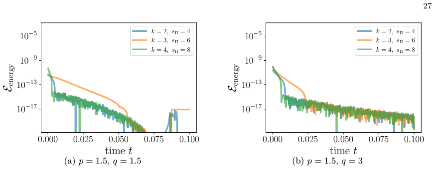
- [Figure 4.2 caption] The caption says 'left, middle' for the convergence histories, but the figure has panels (a), (b), and (c); please refer to the panels explicitly to avoid ambiguity.
- [Section 4.3] The text notes that sQ = 2k is used for the Cahn–Hilliard example because it improves Newton convergence, whereas Section 4.2 uses sQ = k+1. A brief general remark on how sQ is selected in practice would improve reproducibility.
- [References] Reference [GM26] is listed with the arXiv identifier 2603.08656, which appears to contain an impossible date; please verify the identifier.
Circularity Check
No significant circularity: the discrete dissipation inequality in Proposition 3.6 is a direct consequence of the scheme's test-space construction and the stated properties of j and r, not a fitted or self-cited result.
full rationale
The paper's central claim, Proposition 3.6, is verified by an explicit chain of equalities. The proof uses Lemma 3.1 to replace ∂z2H by its projection, then observes that the three components of the chosen test function lie in Wτh, and finally applies Scheme 3.2. The inequality (3.6) follows from the standing assumption (2.3) that r is dissipative and j is skew. No quantity is fitted to a target dissipation value, and no external uniqueness or existence theorem is invoked to make the dissipation inequality true. The scheme is deliberately constructed so that the dissipation identity holds, but that is a design verification, not circularity: the theorem is derived from the stated hypotheses rather than assumed. The paper relies on the authors' prior work for the model class [AS25], the projection technique [GKT25], and technical details of well-definedness and time-stepping [Kar26], but these citations are not load-bearing for the proof of Proposition 3.6; the proof itself is self-contained apart from standard chain-rule and projection arguments. The main gap is the deferred well-posedness of the per-interval nonlinear systems, which affects correctness and applicability but is a separate issue from circularity. There is no evidence that any prediction reduces by construction to its inputs.
Assumptions & free parameters
free parameters (4)
- Quadrature node count sΠ for temporal projection =
sΠ = 2k in all experiments
- Quadrature node count sQ for right-hand side =
sQ = k+1 (circuit) or sQ = 2k (Cahn-Hilliard, doubly nonlinear)
- POD reduced dimensions for Cahn-Hilliard ROM =
5 and 5
- Time scaling θ in manufactured solution for doubly nonlinear example =
θ = 50
assumptions (7)
- domain assumption Assumption 2.1: reflexive Banach spaces X1,X2, Hilbert spaces Z1,Z2,X3 with dense continuous embeddings, and Fréchet differentiable H on an open subset of eX1×eX2.
- domain assumption For admissible states, ∂zi H(z1,z2) ∈ Xi for i = 1,2.
- domain assumption j satisfies ⟨j(v),v⟩ = 0 and r satisfies ⟨r(v),v⟩ ≥ 0 for all v ∈ X.
- domain assumption The continuous system (2.4) admits a unique solution on [0,T] for given u.
- domain assumption The nonlinear systems in Scheme 3.2 admit solutions, and Newton's method converges.
- domain assumption For Proposition 3.14: J11=0, R11=I, J21=R21, J31=R31, det(J33-R33)≠0, V3=I, V1,V2 orthogonal, and ∇H Lipschitz continuous.
- standard math Quadrature weights ωℓ are positive and sum to 1.
Cite this review
Pith. "Pith review of Structure-Preserving Discretization and Model Reduction for Energy-Based Models." pith.science (2026). https://pith.science/paper/2XTAFAWJ
@misc{pith2026250721552,
  author       = {Pith},
  title        = {Pith review of: Structure-Preserving Discretization and Model Reduction for Energy-Based Models},
  year         = {2026},
  howpublished = {\url{https://pith.science/paper/2XTAFAWJ}},
  note         = {Machine review of arXiv:2507.21552}
}
read the original abstract
We investigate discretization strategies for a recently introduced class of energy-based models. The model class encompasses classical port-Hamiltonian systems, generalized gradient flows, and certain systems with algebraic constraints. Our framework combines existing ideas from the literature and systematically addresses temporal discretization, spatial discretization, and model order reduction, ensuring that all resulting schemes are dissipation-preserving in the sense of a discrete dissipation inequality. For this, we use a Petrov--Galerkin ansatz together with appropriate projections. Numerical results for a nonlinear circuit model, the Cahn--Hilliard equation, and a doubly nonlinear parabolic equation illustrate the effectiveness of the approach.
Figures


Figures from the paper (5 more)




Reference graph
Works this paper leans on
-
[1958]
[CH17] E. Celledoni and E. H. Høiseth. Energy-preserving and passivity-consistent numerical discretiza- tion of port-Hamiltonian systems.arXiv preprint 1706.08621,
- [1994]
-
[1996]
[GPBvdS12] S. Gugercin, R. V. Polyuga, C. Beattie, and A. J. van der Schaft. Structure-preserving tangential interpolation for model reduction of port-Hamiltonian systems.Automatica, 48(9):1963–1974,
work page 1963
-
[2019]
[KMS25] P. L. Kinon, R. Morandin, and P. Schulze. Discrete gradient methods for port-Hamiltonian differential-algebraic equations.arXiv preprint 2505.18810,
-
[2025]
Structure-Preserving Generalized Manifold Galerkin Reduction for Port-Hamiltonian Systems
[GM26] S. Glas and H. Mu. Structure-preserving model reduction on manifolds of port-Hamiltonian systems. ArXiv preprint 2603.08656,
-
[2026]
Passivity encoding representations of nonlinear systems
[KBRS24] A. Karsai, T. Breiten, J. Ramme, and P. Schulze. Nonlinear port-Hamiltonian systems and their connection to passivity.arXiv preprint 2409.06256,
Reviewed August 6, 2026 · model on record in the stance chip above.
Discussion (0). Continue with ORCID to comment.