REVIEW 3 major objections 5 minor 47 references
Pulsatile Flows for Simplified Smart Fluids with Variable Power-Law: Analysis and Numerics
T0 review · 3 major / 5 minor · reviewed 2026-08-06 · deepseek-v4-flash
Pith's one-line read This paper proves that pulsatile pipe flows exist for fluids with a position-dependent power-law index, for prescribed flow rate or pressure drop, and that a fully-discrete scheme converges to them.
desk verdict A real variable-exponent extension of the Womersley/Leray line, but the abstract oversells the generality: the convergence theorem needs κ2=0 and the pressure-drop half is left unproved. read the letter →
The pith
A machine-rendered reading of the paper's core claim, the machinery that carries it, and where it could break.
The reading
What carries the argument
The central objects are the reduced scalar problem (3.2) obtained from the fully-developed ansatz, whose stress vector $s(x,a)=\nu(x,|a|^2/2)\,a/2$ inherits coercivity, growth, and strict monotonicity from the original tensor, and the flux-free shift $u=v-\alpha\chi$: an auxiliary function $\chi$ with unit mean over the cross-section absorbs the prescribed flow rate $\alpha$, converting the constrained problem into an equation for $u$ on the zero-mean subspace, with the pressure drop later recovered by $\Gamma=-(\partial_t v,\chi)_\Sigma-(s(\cdot,\nabla v),\nabla\chi)_\Sigma$. Discrete solvability comes from the Edelstein fixed-point theorem (a contraction on a compact ball in the finite-element space) applied to the initial-to-final value map, with the discrete Gronwall lemma in difference form providing the invariant ball. The passage to the continuous problem rests on the strong stability bounds (4.48), which bound the time differences and gradient modulars and hold only when $\kappa_2=0$, enabling a Minty-type monotonicity identification of the weak limit of the stress. The explicit solutions of Section 6 arise by integrating $-\partial_x(|\partial_x v|^{p(x)-2}\partial_x v)=1$ on each interval where $p$ is constant and patching the pieces by continuity of $v$ and of the shear stress.
What would settle it
Take the $\delta$-regularized stress $s(x,a)=(\delta+|a|)^{p(x)-2}a$ with $\delta>0$ and a cross-section where $p$ takes values on both sides of $2$ (so that (s.2) forces $\kappa_2>0$), and compute the discrete solutions of (4.15)–(4.16b) on refining meshes with a genuinely time-dependent flow rate: if the bound on $\|d_\tau v^\tau_h\|_{I\times\Sigma}$ deteriorates as $\tau,h\to 0^+$ or the scheme fails to converge, the stated scope of the theorem is exactly the $\kappa_2=0$ class, whereas if the bound holds, $\kappa_2=0$ is not needed.
Extended reading notes
Core claim
Starting from the fully-developed ansatz $v(t,x)=v(t,x)e_1$, $\pi(t,x)=\Gamma(t)x_1$, the paper reduces the infinite-pipe problem to a $(d-1)$-dimensional scalar problem with stress vector $s(x,a)$ satisfying coercivity, growth, and strict monotonicity assumptions (s.1)–(s.4). Under the additional hypothesis that the coercivity offset $\kappa_2$ in (s.2) vanishes identically on the cross-section, Theorem 4.14 establishes a unique variational solution $(v,\Gamma)$ in $W^{1,2}(I;L^2(\Sigma))\cap L^\infty(I;W_0^{1,p(\cdot)}(\Sigma))\times L^2(I)$ for the flow-rate problem, and the fully-discrete solutions converge weakly to it as time step and mesh size go to zero; Theorem 5.5 makes the analogous claim for the pressure-drop problem, through the same strong-stability machinery. The discrete existence proof is constructive: the Edelstein fixed-point theorem applied to the map sending an initial datum to the final value of the corresponding initial-value problem gives a unique discrete solution and doubles as a Picard algorithm. For a strip with piecewise-constant exponent, the steady problem is solved in closed form, producing Lipschitz velocities patched from power functions, for both even and one-jump non-even exponent profiles; the numerical experiments report the predicted error decay rates and show the reduced one-dimensional model reproducing the interior of a full two-dimensional simulation.
Load-bearing premise
The load-bearing premise is that the coercivity offset $\kappa_2$ in assumption (s.2) is identically zero on the cross-section: the strong stability bound (4.48) that drives the limit passage is proved only in that case, so for stresses such as the $\delta$-regularized model $(\delta+|a|)^{p(x)-2}a$ with $\delta>0$, where $\kappa_2>0$ in general, the paper's existence proof does not apply even though the abstract advertises the full (s.1)–(s.4) class.
Editorial extensions
If this is right
- Time-periodic fully-developed flows with prescribed flow rate or prescribed pressure drop exist and are unique for variable-exponent fluids in the $\kappa_2=0$ class, in particular for the pure $p(x)$-Laplacian-type stress $s(x,a)=|a|^{p(x)-2}a$.
- Because the existence proof is constructive, the same discrete scheme—backward differences, finite elements, Picard iteration on the initial datum—can be used directly as a solver, with weak convergence guaranteed.
- The closed-form steady solutions give variable-exponent analogues of Hagen–Poiseuille flow, including asymmetric exponent profiles, usable as benchmarks in CFD codes.
- All $p(x)\in(1,+\infty)$ are treated uniformly and no auxiliary Newtonian term is needed, yielding an alternative proof of the constant-exponent results and fresh insight into the Newtonian case.
- The reduced $(d-1)$-dimensional model matches the interior of the full $d$-dimensional simulation in the reported experiments, supporting the fully-developed reduction as a reliable computational shortcut.
Reading between the lines
- The abstract claims existence for the whole (s.1)–(s.4) class, but the proof as written delivers it only for $\kappa_2=0$; whether the $\delta$-regularized model admits time-periodic solutions is therefore still open on the evidence of this paper.
- Because $\delta$-regularization is the standard device in numerical implementations, a stability estimate that absorbs $\kappa_2$ (or a Leray–Schauder-type argument) would close the gap; the paper's own variable-exponent numerics use the unregularized stress, so they do not exercise the gap.
- A testable extension suggested by Section 6: for rectangular ducts with $p$ depending on a single coordinate, the same one-dimensional patched solutions should carry over (as the paper hints in Remark 6.1), which comparison numerics could verify.
Editorial analysis
A structured set of objections, weighed in public.
Referee Report
Summary. The paper studies fully-developed, time-periodic, shear-dependent flows of p(x)-power-law fluids in an infinite pipe, for both prescribed flow rate and prescribed pressure drop. The main theoretical contribution is a fully-constructive existence proof for variational solutions via a fully-discrete finite-difference/finite-element scheme, together with explicit time-independent benchmark solutions for piecewise-constant variable exponents and numerical experiments comparing the reduced 1D model with a direct 2D approximation.
Significance. If the results are established at the claimed level of generality, the paper would extend the Womersley/Leray flow-rate and pressure-drop existence theory from constant p and from Navier-Stokes to variable-exponent p(x)-fluids for all p(x) in (1,∞), without an auxiliary Newtonian term. The fully-discrete constructive proof, the explicit benchmark solutions, and the numerical comparison between the reduced and full models are all valuable and largely reproducible contributions. However, as detailed below, the generality actually proved in the manuscript is narrower than the abstract's claim, and two load-bearing parts of the proof are either conditional on κ2=0 or omitted.
major comments (3)
- [§4, Lemma 4.13 and Theorem 4.14; §2.2 (S.2)/§3 (s.2)] The convergence and existence theorem for the flow-rate problem is proved only under the assumption κ2=0 a.e. in Σ, as stated at the beginning of Lemma 4.13 and in Theorem 4.14. This excludes the paper's own motivating example, the (p(·),δ)-structure s(x,a)=(δ+|a|)^{p(x)-2}a with δ>0, whenever p(x)<2 on a set of positive measure, because for such x the quotient s(x,a)·a/|a|^{p(x)} = (δ+|a|)^{p(x)-2}|a|^{2-p(x)} tends to 0 as |a|→0, so (s.2) cannot hold with κ2=0. The proof of Lemma 4.13 uses κ2=0 precisely where the lower bound of the potential V in Lemma 3.3(iii) is needed to obtain the strong stability estimates (4.48), which in turn provide the compactness and the Minty-type identification in Theorem 4.14. The abstract and Section 1, however, advertise existence for the full class (S.1)-(S.4) and for the prototype (1.4) with δ≥0. This is a load-bearing scope mismatch: the main theorem should either be extended to κ2>0 or the claims in the abstract and introduction should be restricted accordingly.
- [§5, Lemma 5.4 and Theorem 5.5] The pressure-drop half of the central claim is not established within the manuscript: Lemma 5.4 (strong stability) and Theorem 5.5 (weak convergence and existence) are stated, but their proofs are left to the interested reader. The abstract and the introduction promise existence of time-periodic solutions with assigned pressure drop, so this is not a peripheral remark. At minimum, the authors need to provide the proofs or state the pressure-drop result as conditional/deferred with a precise reference to a future work.
- [§4, Eq. (4.38) and Lemma 4.11] Equation (4.38) contains a sign inconsistency in the application of the discrete Gronwall lemma. The text applies Lemma 4.11 with λ = -κ1/(cP 2^{p+}) in (4.37), but the resulting bound in (4.38) is written with (1+λτ)^m and c1/(-λτ). For λ<0, the factor 1+λτ is smaller than 1, and the second term {1 - 1/(1+λτ)^m} c1/(-λτ) is negative, which cannot serve as an upper bound. The correct expression from Lemma 4.11 would involve (1-λτ)^m = (1+|λ|τ)^m and a positive second term. This estimate is used to prove that the fixed-point operator maps the ball B^τ_h into itself, so the error affects the constructive existence argument in Lemma 4.9. The issue appears fixable by correcting the sign convention, but as written it is a load-bearing inconsistency in the discrete existence proof.
minor comments (5)
- [§4, Lemma 4.8] In Lemma 4.8 the phrase 'in the sense of Definition 4.4' appears twice; the flux-free discrete formulation is Definition 4.7, not Definition 4.4.
- [§4, Eq. (4.57c)] The convergence stated as '(τ → +∞)' should read '(τ → 0+)'.
- [§6, Eq. (6.10)] The sign assumption on ∂xv in (6.10) is imposed a priori. Since the goal is to construct explicit solutions, this is acceptable, but it would help to state explicitly that this sign condition is an ansatz used to select a branch of the solution, not a consequence of the boundary-value problem.
- [§7.3, stress-tensor scaling] The formula for the reduced stress vector in Section 7.3, displayed as '2^{2+p(x)/2}', is typographically ambiguous and the exponent appears algebraically wrong; the factor should be checked and stated without ambiguity, because the numerical comparison uses this scaling.
- [§1 and §2] The paper repeatedly cites [6,7,27] for technical lemmas and for the convergence-rate discussion in Remark 4.12. The citations are used appropriately, but a sentence in Remark 4.12 clarifying which results are taken from [6] and which are new to this paper would improve readability.
Circularity Check
No circular derivation: the central existence proof is self-contained, though its advertised scope is narrower than the abstract (κ2=0 assumption) and the pressure-drop half is left to the reader.
full rationale
The central claim, Theorem 4.14, is proved by a genuinely constructive route: the fully-discrete problem is solved with an external Edelstein fixed-point theorem, stability estimates follow from monotonicity and coercivity, and the weak limit is identified by a Minty-type argument. No parameter is fitted to data and then renamed a prediction; the numerical experiments are tested against independently constructed explicit solutions, not against quantities used to calibrate the scheme. The paper does cite the authors' own works [6,7,27], but only for a standard variable-exponent Young inequality and for optional convergence-rate estimates in Remark 4.12; these are not the load-bearing basis of the main theorem, and the main existence proof does not reduce to a prior result of the same authors. The most serious issue is a proof-scope gap, not circularity: Lemma 4.13 and Theorem 4.14 explicitly assume 'κ2 = 0 a.e. in Σ in (s.2)', while the abstract's prototypical model (δ+|a|)^{p(x)-2}a with δ>0 and p(x)<2 violates this assumption, so existence for the full (s.1)-(s.4) class advertised in the abstract is not established. Similarly, Theorem 5.5 for assigned pressure drop is stated with 'The proofs ... are left to the interested reader', so that half of the abstract's claim is not proven in the preprint. These are scope and rigor concerns that should be reported as correctness risk, but they do not make the derivation circular; the argument that is actually given is self-contained.
Assumptions & free parameters
assumptions (6)
- domain assumption Stress tensor satisfies (s.1)-(s.4): Carathéodory, coercivity with κ1>0, growth with κ3≥0, strict monotonicity
- domain assumption Variable exponent p ∈ P∞(Σ) with p_- > 1
- standard math The projection operator Π_h satisfies Assumption 2.2 (P1 inclusion, W^{1,1}-stability)
- standard math Edelstein fixed point theorem and discrete Gronwall lemma
- standard math Existence of χ ∈ W^{1,p(·)}_0(Σ) with (χ,1)_Σ=1
- ad hoc to paper Sign assumption (6.10) for the even explicit solution
Cite this review
Pith. "Pith review of Pulsatile Flows for Simplified Smart Fluids with Variable Power-Law: Analysis and Numerics." pith.science (2026). https://pith.science/paper/AH3PPZAE
@misc{pith2026250722449,
  author       = {Pith},
  title        = {Pith review of: Pulsatile Flows for Simplified Smart Fluids with Variable Power-Law: Analysis and Numerics},
  year         = {2026},
  howpublished = {\url{https://pith.science/paper/AH3PPZAE}},
  note         = {Machine review of arXiv:2507.22449}
}
abstract
We study the fully-developed, time-periodic motion of a shear-dependent non-Newtonian fluid with variable exponent rheology through an infinite pipe $\Omega:= \mathbb{R}\times \Sigma\subseteq \mathbb{R}^d$, $d\in \{2,3\}$, of arbitrary cross-section $\Sigma\subseteq \mathbb{R}^{d-1}$. The focus is on a generalized $p(\cdot)$-fluid model, where the power-law index is position-dependent (with respect to $\Sigma$), $\textit{i.e.}$, a function $p\colon \Sigma\to (1,+\infty)$. We prove the existence of time-periodic solutions with either assigned time-periodic flow-rate or pressure-drop, generalizing known results for the Navier-Stokes and for $p$-fluid equations. In addition, we identify explicit solutions, relevant as benchmark cases, especially for electro-rheological fluids or, more generally, $\textit{`smart fluids'}$. To support practical applications, we present a fully-constructive existence proof for variational solutions by means of a fully-discrete finite-differences/-elements discretization, consistent with our numerical experiments. Our approach, which unifies the treatment of all values of $p(\overline{x})\in (1,+\infty)$, $\overline{x}\in \Sigma$, without requiring an auxiliary Newtonian term, provides new insights even in the constant exponent case. The theoretical findings are reviewed by means of numerical experiments.
Figures
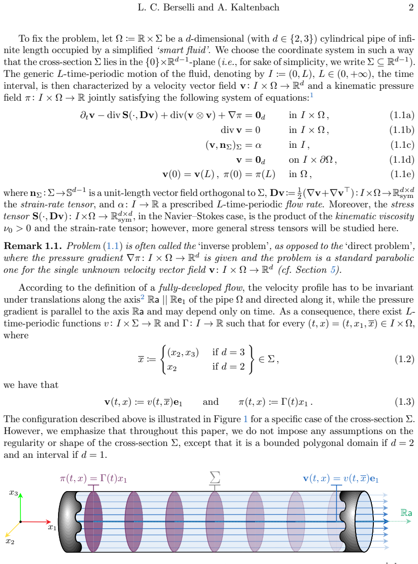


Figures from the paper (9 more)


Reference graph
Works this paper leans on
-
[1]
B. Amaziane, L. Pankratov, and A. Piatnitski, Nonlinear flow through double porosity media in variable exponent Sobolev spaces, Nonlinear Anal. Real World Appl. 10 no. 4 (2009), 2521–2530. doi:10.1016/j.nonrwa.2008.05.008
-
[2]
P. R. Amestoy, I. S. Duff, J.-Y. L’Excellent, and J. Koster, A fully asynchronous multifrontal solver using distributed dynamic scheduling, SIAM J. Matrix Anal. Appl. 23 no. 1 (2001), 15–41. doi:10.1137/S0895479899358194
-
[3]
S. N. Antontsev and J. F. Rodrigues , On stationary thermo-rheological viscous flows, Ann. Univ. Ferrara Sez. VII Sci. Mat. 52 no. 1 (2006), 19–36. doi:10.1007/s11565-006-0002-9
-
[4]
S. Banach , Sur les op´ erations dans les ensembles abstraits et leur application aux ´ equations int´ egrales.,Fundam. Math. 3 (1922), 133–181. doi:10.4064/fm-3-1-133-181
-
[5]
Behera, Advanced Materials, Springer International Publishing, 06 2021
A. Behera, Advanced Materials, Springer International Publishing, 06 2021. doi:10.1007/978-3-030- 80359-9
-
[6]
L. C. Berselli and A. Kaltenbach, Error analysis for a finite element approximation of the steady p(·)-Navier–Stokes equations, IMA J. Numer. Anal. (2024), drae082. doi:10.1093/imanum/drae082
-
[7]
L. C. Berselli and A. Kaltenbach, Convergence analysis for a fully-discrete finite element approximation of the unsteady p(·, ·)-Navier-Stokes equations, Numer. Math. 157 no. 2 (2025), 573–627. doi:10.1007/s00211-025-01450-1
-
[8]
L. C. Berselli , P. Miloro , A. Menciassi , and E. Sinibaldi , Exact solution to the inverse Womersley problem for pulsatile flows in cylindrical vessels, with application to magnetic particle targeting, Appl. Math. Comput. 219 no. 10 (2013), 5717–5729. doi:10.1016/j.amc.2012.11.071
Show all 47 references
-
[9]
L. C. Berselli and M. Romito, On Leray’s problem for almost periodic flows, J. Math. Sci., Tokyo 19 no. 1 (2012), 69–130
2012
-
[10]
Blomgren, T
P. Blomgren, T. Chan, P. Mulet, and C. Wong, Total variation image restoration: numerical methods and extensions, in Proc. - Int. Conf. Image Process. ICIP , 3, 1997, pp. 384–387 vol.3. doi:10.1109/ICIP.1997.632128
1997
-
[11]
Breit, L
D. Breit, L. Diening, and S. Schwarzacher, Finite Element Approximation of the p(·)-Laplacian, SIAM J. Numer. Anal. 53 no. 1 (2015), 551–572. doi:10.1137/130946046. Pulsatile Flows of Simplified Smart Fluids 35
2015 doi
-
[12]
Bridges, S
C. Bridges, S. Karra, and K. R. Rajagopal, On modeling the response of the synovial fluid: unsteady flow of a shear-thinning, chemically-reacting fluid mixture, Comput. Math. Appl. 60 no. 8 (2010), 2333–2349. doi:10.1016/j.camwa.2010.08.027
2010 doi
-
[13]
I. A. Brigadnov and A. Dorfmann, Mathematical modeling of magnetorheological fluids, Contin. Mech. Thermodyn. 17 no. 1 (2005), 29–42. doi:10.1007/s00161-004-0185-1
2005 doi
-
[14]
Cekic , A
B. Cekic , A. Kalinin , R. Mashiyev , and M. A vci, Lp(x)(Ω)-estimates of vector fields and some applications to magnetostatics problems, J. Math. Anal. 389 no. 2 (2012), 838–851. doi:10.1016/j.jmaa.2011.12.029
2012 doi
-
[15]
Diening and M
L. Diening and M. R˚uˇziˇcka, Interpolation operators in Orlicz–Sobolev spaces, Numer. Math. 107 no. 1 (2007), 107–129. doi:10.1007/s00211-007-0079-9
2007 doi
-
[16]
Diening , P
L. Diening , P. Harjulehto , P. H ¨ast¨o, and M. R˚uˇziˇcka, Lebesgue and Sobolev spaces with variable exponents, Lect. Notes Math. 2017, Berlin: Springer, 2011. doi:10.1007/978-3-642-18363-8
2017 doi
-
[17]
Droniou, Int´ egration et Espaces de Sobolev ` a Valeurs Vectorielles., April 2001
J. Droniou, Int´ egration et Espaces de Sobolev ` a Valeurs Vectorielles., April 2001
2001
-
[18]
Edelstein, On fixed and periodic points under contractive mappings, J
M. Edelstein, On fixed and periodic points under contractive mappings, J. Lond. Math. Soc. 37 (1962), 74–79. doi:10.1112/jlms/s1-37.1.74
1962 doi
-
[19]
Emmrich, Discrete versions of Gronwall’s lemma and their application to the numerical analysis of parabolic problems, Tech
E. Emmrich, Discrete versions of Gronwall’s lemma and their application to the numerical analysis of parabolic problems, Tech. Report 637, Institute of Mathematics, Technical University of Berlin,
-
[20]
Ern and J.-L
A. Ern and J.-L. Guermond, Finite elements I. Approximation and interpolation , Texts Appl. Math. 72, Cham: Springer, 2020. doi:10.1007/978-3-030-56341-7
2020 doi
-
[21]
Formaggia, A
L. Formaggia, A. Veneziani, and C. Vergara, Flow rate boundary problems for an incompressible fluid in deformable domains: formulations and solution methods, Comput. Methods Appl. Mech. Eng. 199 no. 9-12 (2010), 677–688. doi:10.1016/j.cma.2009.10.017
2010 doi
-
[22]
Gajewski, K
H. Gajewski, K. Gr ¨oger, and K. Zacharias, Nichtlineare Operatorgleichungen und Operatordif- ferentialgleichungen, Math. Lehrb¨ ucher Monogr., II. Abt., Math. Monogr. 38, Akademie-Verlag, Berlin, 1974
1974
-
[23]
G. P. Galdi , Mathematical problems in classical and non-Newtonian fluid mechanics, in Hemody- namical flows, Oberwolfach Semin. 37, Birkh¨ auser, Basel, 2008, pp. 121–273. doi:10.1007/978-3- 7643-7806-6 3
2008 doi
-
[24]
G. P. Galdi and C. R. Grisanti , Womersley flow of generalized Newtonian liquid, Proc. R. Soc. Edinb., Sect. A, Math. 146 no. 4 (2016), 671–692. doi:10.1017/S0308210515000736
2016 doi
-
[25]
Hagen, Ueber die Bewegung des Wassers in engen cylindrischen R¨ ohren,Ann
G. Hagen, Ueber die Bewegung des Wassers in engen cylindrischen R¨ ohren,Ann. Phys. 122 no. 3 (1839), 423–442. doi:10.1002/andp.18391220304
-
[26]
Harjulehto, P
P. Harjulehto, P. H¨ast¨o, and M. Koskenoja, The Dirichlet energy integral on intervals in vari- able exponent Sobolev spaces, Z. Anal. Anwend. 22 no. 4 (2003), 911–923. doi:10.4171/ZAA/1179
2003 doi
-
[27]
Kaltenbach, Pseudo-monotone operator theory for unsteady problems with variable exponents , Lect
A. Kaltenbach, Pseudo-monotone operator theory for unsteady problems with variable exponents , Lect. Notes Math. 2329, Cham: Springer, 2023. doi:10.1007/978-3-031-29670-3
2023 doi
-
[28]
Logg, K.-A
A. Logg, K.-A. Mardal, and G. Wells (eds.), Automated solution of differential equations by the finite element method. The FEniCS book , Lect. Notes Comput. Sci. Eng. 84, Berlin: Springer,
-
[29]
M ´alek, J
J. M ´alek, J. Ne ˇcas, M. Rokyta, and M. R˚uˇziˇcka, Weak and Measure-valued Solutions to Evolutionary PDEs , Appl. Math. Comput. 13, Chapman & Hall, London, 1996
1996
-
[30]
J. L. M. Poiseuille , Recherches exp´ erimentales sur le mouvement des liquides dans les tubes de tr` es-petits diam` etres,M´ emoires pr´ esent´ es par divers savants ` a l’Acad´ emie Royale des Sciences de l’Institut de France 9 (1846), 433–544
-
[31]
Quarteroni, Mathematical modelling of the cardiovascular system, in Proceedings of the international congress of mathematicians, ICM 2002, Beijing, China, August 20–28, 2002
A. Quarteroni, Mathematical modelling of the cardiovascular system, in Proceedings of the international congress of mathematicians, ICM 2002, Beijing, China, August 20–28, 2002. Vol. III: Invited lectures, Beijing: Higher Education Press; Singapore: World Scientific/distributo...
2002
-
[32]
Roub´ıˇcek, Nonlinear partial differential equations with applications , 2nd ed
T. Roub´ıˇcek, Nonlinear partial differential equations with applications , 2nd ed. ed., ISNM, Int. Ser. Numer. Math. 153, Basel: Birkh¨ auser, 2013. doi:10.1007/978-3-0348-0513-1
2013 doi
-
[33]
R˚uˇziˇcka, Electrorheological fluids: modeling and mathematical theory , Lect
M. R˚uˇziˇcka, Electrorheological fluids: modeling and mathematical theory , Lect. Notes Math. 1748, Berlin: Springer, 2000. doi:10.1007/BFb0104029
-
[34]
L. R. Scott and S. Zhang, Finite element interpolation of nonsmooth functions satisfying boundary conditions, Math. Comput. 54 no. 190 (1990), 483–493. doi:10.2307/2008497. L. C. Berselli and A. Kaltenbach 36
1990 doi
-
[35]
Taylor and P
C. Taylor and P. Hood, A numerical solution of the Navier-Stokes equations using the finite element technique, Comput. Fluids 1 (1973), 73–100 (English). doi:10.1016/0045-7930(73)90027-3
1973 doi
-
[36]
Temam, Navier-Stokes equations
R. Temam, Navier-Stokes equations. Theory and numerical analysis , North-Holland Publishing Co., Amsterdam-New York-Oxford, 1977, Studies in Mathematics and its Applications, Vol. 2
1977
-
[37]
Beir ˜ao da Veiga , Time-periodic solutions of the Navier-Stokes equations in unbounded cylindrical domains-Leray’s problem for periodic flows, Arch
H. Beir ˜ao da Veiga , Time-periodic solutions of the Navier-Stokes equations in unbounded cylindrical domains-Leray’s problem for periodic flows, Arch. Ration. Mech. Anal. 178 no. 3 (2005), 301–325. doi:10.1007/s00205-005-0376-3
2005 doi
-
[38]
Veneziani and C
A. Veneziani and C. Vergara , Flow rate defective boundary conditions in haemodynamics simulations, Int. J. Numer. Methods Fluids 47 no. 8-9 (2005), 803–816. doi:10.1002/fld.843
2005 doi
-
[39]
Veneziani and C
A. Veneziani and C. Vergara, An approximate method for solving incompressible Navier-Stokes problems with flow rate conditions, Comput. Methods Appl. Mech. Eng. 196 no. 9-12 (2007), 1685–1700. doi:10.1016/j.cma.2006.09.011
2007 doi
-
[40]
J. R. Womersley , Method for the calculation of velocity, rate of flow and viscous drag in arteries when the pressure gradient is known, J. Physiol. 3 no. 127 (1955), 553–563. doi:10.1113/jphysiol.1955.sp005276
1955 doi
-
[41]
Zeidler, Nonlinear functional analysis and its applications
E. Zeidler, Nonlinear functional analysis and its applications. II/A: Linear monotone operators. Transl. from the German by the author and by Leo F. Boron , New York etc.: Springer-Verlag, 1990
1990
-
[42]
Zeidler, Nonlinear functional analysis and its applications
E. Zeidler, Nonlinear functional analysis and its applications. II/B: Nonlinear monotone operators. Transl. from the German by the author and by Leo F. Boron , New York etc.: Springer-Verlag, 1990
1990
-
[43]
V. V. Zhikov, Averaging of functionals of the calculus of variations and elasticity theory, Math. USSR, Izv. 29 (1987), 33–66. doi:10.1070/IM1987v029n01ABEH000958
1987 doi
-
[44]
V. V. Zhikov, Meyer-type estimates for solving the nonlinear Stokes system, Differ. Uravn. 33 no. 1 (1997), 107–114
1997
-
[45]
V. V. Zhikov, On some variational problems, Russ. J. Math. Phys. 5 no. 1 (1997), 105–116. A. Approximation and boundedness properties of χh In this short appendix, we intend to catch up proving the approximation and stability properties (4.18a),(4.18b) of the function χh ∈ Vh,...
1997
-
[1999]
doi:10.14279/depositonce-14714
-
[2012]
doi:10.1007/978-3-642-23099-8
Reviewed August 6, 2026 · model on record in the stance chip above.
Discussion (0). Sign in to comment.