REVIEW 5 major objections 7 minor 40 references
A visual analytics tool for taxonomy-based trajectory data exploration
T0 review · 5 major / 7 minor · reviewed 2026-08-06 · deepseek-v4-flash
Pith's one-line read A four-zone outlier workflow turns unlabeled tracks into behavior labels, statistical drivers, and map-visible turning points.
desk verdict A useful interactive operationalization of TUMD, but the case-study behavioral claims outrun the validation. read the letter →
The pith
A machine-rendered reading of the paper's core claim, the machinery that carries it, and where it could break.
The reading
What carries the argument
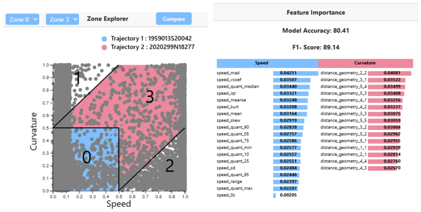
The load-bearing device is the four-zone decision boundary computed from the two outlier scores assigned to each trajectory, one per selected taxonomy dimension. Scores are produced by Distance-Based Outlier Scoring (DBOS), which measures how isolated each trajectory is from its neighbors in feature space; the zones partition the unit square by whether each score exceeds 0.5 and by linear inequalities, yielding the labels "no significant behavior," "behavior of the y dimension only," "behavior of the x dimension only," and "hybrid behavior." A random forest trained on the points inside two selected zones supplies feature importance rankings of 72 statistical variables, and the selected variables trigger focused 2D heatmap and 3D wall views of short trajectory segments. This mechanism is what carries the argument from coordinates to behavior categories to inspectable locations in space and time.
What would settle it
Take a labeled or expert-annotated subset of trajectories, such as known fox behaviors or cyclone segments with documented sharp turns, and compare their assigned zone labels against the measured acceleration, curvature, and angle profiles. If trajectories in the acceleration zone are not systematically more steady in acceleration than curvature-zone trajectories, or if hybrid-zone cyclones do not show the predicted pivot angles, the score-to-behavior mapping is falsified.
Extended reading notes
Core claim
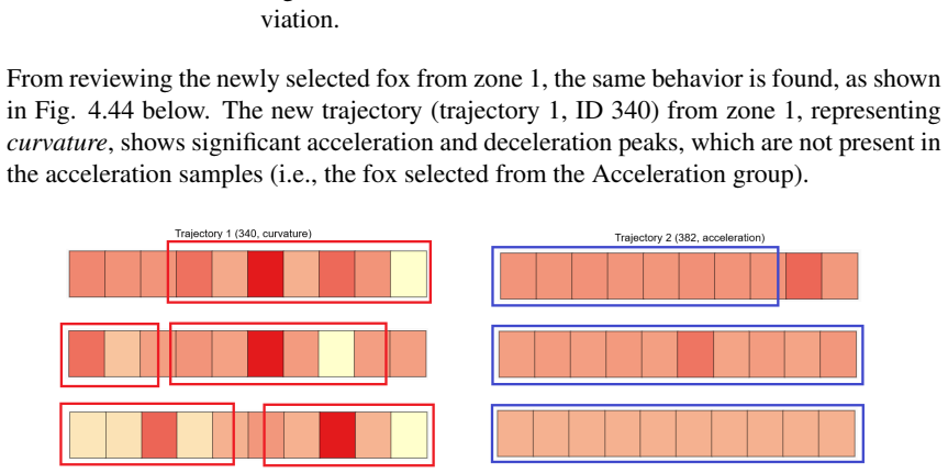
The central claim is that unlabeled trajectories can be described by a small taxonomy, with two top-level groups, Geometric and Kinematic, subdivided into Curvature, Indentation, Acceleration, and Speed, and that outlier scores on any pair of these dimensions create meaningful behavioral classes. Distance-Based Outlier Scores in $[0,1]$ place each trajectory in one of four zones: neither dimension significant, only the first, only the second, or a hybrid of both. Comparing zones with a random-forest feature importance model then names the specific statistical variables, such as acceleration standard deviation, distance geometry signatures, and angle kurtosis, that separate the behaviors. The paper's case studies report that foxes labeled acceleration-based showed steady acceleration while curvature-based foxes showed acceleration peaks and deceleration, and that a cyclone labeled hybrid curvature-indentation owed its shape to two pivot angles of 153 and 135 degrees. The authors take these results to show that complex movement data can be analyzed in detail from raw input to semantic labels through iterative visual-analytic steps.
Load-bearing premise
The entire interpretation rests on one premise: that a DBOS outlier score above 0.5 on a taxonomy dimension really means the trajectory exhibits that behavior, and no ground-truth labels, expert validation, or external benchmark support this mapping.
Editorial extensions
If this is right
- An analyst can begin with no labels and still group trajectories into behavior classes, because the taxonomy and zone boundaries supply the categories.
- The same pipeline should transfer to any movement dataset with speed, acceleration, angle, distance, and bearing features, not just animals and storms.
- Each behavioral assignment is traceable to a ranked list of statistical variables and to specific map points, so pattern claims can be inspected rather than taken on faith.
- The cyclic workflow of overview, zone comparison, variable selection, map view, and re-selection provides a concrete procedure for exploratory data analysis on movement data.
Reading between the lines
- A testable extension the paper does not run: use the full fox dataset to compare acceleration variance between zone-labeled acceleration and curvature foxes; the claimed steady-versus-peaky difference should reproduce without any new labels.
- The paper's fixed 0.5 zone threshold is an assumption that could be re-examined; datasets with very dense or very sparse outlier scores may need a data-dependent threshold for the four labels to remain meaningful.
- If the zone-to-behavior mapping is validated, the workflow could replace hand-built anomaly rules in vessel traffic or disease-spread monitoring, where raw tracks are abundant but labels are scarce.
- The authors' angle findings for the cyclone suggest a specific meteorological test: check whether the 153-degree and 135-degree pivot points coincide with documented rapid direction changes or steering-flow shifts in the storm's history.
Signed reviews
Editorial analysis
A structured set of objections, weighed in public.
Referee Report
Summary. The paper presents a visual analytics tool for exploring spatio-temporal trajectory data through a taxonomy-based, multi-level workflow. The pipeline consists of data preprocessing, selection of taxonomy combinations (Kinematic/Geometric and their subdivisions), DBOS-based outlier scoring in a four-zone decision boundary, random forest feature importance for zone comparisons, and linked 2D/3D map visualizations with trajectory sampling. The tool is demonstrated on two case studies: Arctic fox trajectories and tropical cyclone tracks. The authors claim the tool successfully labels trajectories into behavioral groups (e.g., acceleration-based vs. curvature-based) and that the case studies reveal patterns such as constant acceleration for acceleration-labeled foxes and high-angle pivot points for hybrid cyclone trajectories.
Significance. If the central claims were fully supported, the paper would be a useful contribution to visual analytics for movement data: it provides a concrete, interactive implementation of the TUMD taxonomy, a detailed workflow linking low-level statistical features to high-level visual abstractions, and two real-world case studies with publicly sourced datasets. The step-by-step methodology and the explicit integration of DBOS zones with random forest feature importance are clearly described and could serve as a blueprint for similar tools. The authors are also transparent about several limitations, including the absence of user studies and the disclaimer that the system does not provide automated semantic interpretation. However, the significance of the empirical findings is substantially weakened by the circularity between zone construction and feature importance, the lack of ground-truth validation for behavioral labels, and the reliance on a small number of hand-picked trajectories for the main patterns.
major comments (5)
- [3.2.4, 3.2.5, Algorithm 1, and Section 4.1.1] The zone labels that drive all case-study conclusions are definitional artifacts of the same features later used for confirmation. Algorithm 1 defines Zone 1 as 'y > 0.5 and x < (y - 0.5)' and Zone 2 as 'x > 0.5 and y < (x - 0.5)' using DBOS scores computed from the movement features. Section 3.2.5 then runs a random forest on the same feature families to produce feature importance, and the case studies (e.g., Section 4.1.1) interpret the results as 'acceleration-based behavior' and 'curvature-based behavior.' Consequently, the reported F1-scores (e.g., 100% in Fig. 4.36) measure how separable the zones are under the features that defined them, not whether the zones correspond to real behavioral distinctions. The authors should either provide external validation (e.g., expert labels, held-out data, or comparison with known ground-truth behaviors) or explicitly reframe the conclusions as properties of the data-derived zones rather than of the foxes or cyclones themselves.
- [1.6 and Section 4] The paper's own scope statement in Section 1.6 disclaims automated semantic interpretation and domain-specific meaning attribution, yet Sections 4.1 and 4.2 repeatedly assign behavioral semantics to the zones, e.g., 'foxes labeled as having acceleration-based behavior' and 'hybrid Geometric behavior (Curvature and Indentation combined).' No ground-truth labels, expert validation, or external benchmark are introduced anywhere. This makes the behavioral claims unsupported. The case-study conclusions should be presented as exploratory observations about the tool's output, not as validated descriptions of animal or cyclone behavior, unless a validation step is added.
- [4.1.1, Figs. 4.40, 4.44, 4.48] The central pattern in Case Study 1, that foxes in the acceleration zone show 'constant, steady acceleration' while those in the curvature zone show peaks and sudden deceleration, rests on visual inspection of three hand-picked comparisons involving only four individual foxes (IDs 352, 382, 340, 428). The paper states that '9 additional comparisons were performed' but does not report them, and no quantitative summary over all trajectories in each zone (e.g., acceleration variance, number of peaks, or a statistical test) is provided. To support the claimed dichotomy, the authors should report aggregated statistics over all trajectories in each zone and, ideally, perform a statistical comparison between zones.
- [4.2.1, Table 4.1] There is an internal inconsistency in the angle-based evidence for the cyclone case study. The text claims that Trajectory 2 (zone 2, curvature-only) had 'low angle values overall,' but Table 4.1 reports an angle of 180° for Quantile 75 for Trajectory 2, which is actually the highest value in the table and larger than Trajectory 1's 153°. Furthermore, the paper does not define the angle convention (e.g., interior turning angle vs. direction change), which is essential for interpreting whether a 180° value represents a significant directional change or a straight path. This undermines the specific conclusion that the hybrid trajectory is uniquely characterized by high indentation angles.
- [3.5] The random forest feature importance is used as evidence for zone characterization, but the paper reports only accuracy and F1-score, with no confidence intervals, cross-validation details, or statistical significance testing. Given that the model uses the same features that define the zones, the high accuracy is not surprising; reporting only point estimates without quantifying uncertainty is inadequate for the strength of the claims made.
minor comments (7)
- [Abstract] The abstract states that foxes are 'further categorized into Curvature and Acceleration groups,' but the taxonomy also includes Speed and Indentation, which are used in the study; this phrasing is misleading and should be revised.
- [3.2.3] The text refers to 'combination number 3, Acceleration and Speed' as an example, but the numbered list shows that Acceleration and Speed is combination 2. Also, 'Curvature and Speed' appears twice in the list (items 4 and 6); the second instance should be a different combination.
- [3.2.4] The axis assignments for the decision-boundary plot are described in the text (Kinematic on x, Geometric on y), but Algorithm 1 uses generic x and y without specifying which taxonomy parameter is assigned to which axis in a given selection. Please make the coordinate convention explicit and consistent with Fig. 3.9.
- [4.1] In the description of Fig. 4.30, the text says 'the 6th entry present a peak of acceleration (0,0259, Fig. 4.30, bottom left shown in strong red color)' and 'great deceleration (-0.0082, Fig. 4.30, bottom right shown with light yellow color)'; the decimal comma in '0,0259' should be a decimal point for consistency.
- [5] The discussion repeatedly uses the phrase 'correctly identified' and 'correctly categorized' to describe zone assignments, but without ground truth this terminology is too strong; it should be replaced with language such as 'assigned by the outlier score' or 'grouped by the algorithm.'
- [4.2] In Section 4.2, the text first refers to Trajectory 1 as being from zone 0 (no significant behavior) and then later, in the same paragraph, states that 'the outlier score distinction for hybrid behavior was correctly representational for speed and curvature together'; this seems to conflate the initial Speed-Curvature iteration with the later Curvature-Indentation iteration. Please clarify the narrative.
- [General] The paper mentions that the tool is open-sourced, but no repository link or code availability statement is provided in the manuscript. If the tool is intended to be reusable, a link or a separate availability section should be included.
Circularity Check
Zone labels are defined by DBOS thresholds on the same feature families that the feature-importance step and case-study conclusions then 'discover', so the central behavioral findings are partly restatements of the label construction.
-
self definitional
[Section 3.2.4, Algorithm 1 and zone definitions]
"Zone 2: The trajectory points within zone 2 present a score above 0.5 for the x parameters, while the score for the y parameter must satisfy the following linear inequality: y <(x − 0.5). This means that the behavior for the trajectories lying in that zone is mainly due to the element selected as x only."
The 'behavior' labels are not independent categories: a trajectory is called acceleration-based (zone 2 in the Acceleration–Curvature combination) exactly when its DBOS acceleration score exceeds 0.5 and its curvature score is below x−0.5. Later statements such as 'those foxes within the acceleration group ... were often steady and consistent in their acceleration' are re-descriptions of this thresholding rule, not new empirical discoveries. No ground-truth labels or expert validation are introduced (Sec. 1.6), so the semantic mapping from zone to behavior is supplied by the same score that defines the zone.
-
fitted input called prediction
[Section 3.2.5 and Section 4.1 (zone 1 vs zone 2 comparison)]
"Such a comparison is done by implementing a feature importance algorithm, which will analyze the trajectories from the zones selected, effectively deriving the highest contributing features for a trajectory to have been categorized as a member of such a zone."
The random forest is trained to separate zones whose labels were created by thresholding DBOS scores computed from the very 72 statistical variables that feature importance later ranks. In the Acceleration vs Curvature comparison, the top acceleration variables (Acceleration Mean, Acceleration Quantile 95, Acceleration Standard Deviation, etc.) are the same feature family used to define zone 2. The reported F1-scores of 80–100% therefore certify separability of the labels from their own construction features; they do not validate any independent behavioral distinction.
1 more flagged steps
-
self definitional
[Section 4.2, first iteration (Speed–Curvature analysis)]
"This further promotes that the outlier score distinction for hybrid behavior was correctly representational for speed and curvature together, as speed is significant in terms of the highest speed achieved, while curvature and the straightness of the trajectory had a relative impact on it."
The outlier-score 'distinction' is validated by the same speed and curvature features that generated the scores: the trajectory was placed in zone 3 because its speed and curvature scores were high, and the visual check then finds high speed and straightness. This is a self-consistency check between a definition and its instance, not an external confirmation.
full rationale
The core methodological chain is partially circular. Algorithm 1 defines the four zones purely by thresholding DBOS outlier scores on the selected taxonomy parameters, and DBOS is computed from the same movement-feature families (speed, acceleration, curvature, indentation-related angles) that the random forest feature-importance step subsequently ranks to 'explain' zone membership. The case-study conclusions then read behavioral semantics directly from those zone labels: foxes in the high-acceleration zone are described as having constant, steady acceleration, while foxes in the high-curvature zone are described as having acceleration peaks; cyclone trajectories in the hybrid zone are described as having both high curvature and high indentation angles. Each of these is a restatement of the zone-construction criterion rather than evidence from independent ground truth. The paper itself disclaims automated semantic interpretation in Section 1.6, which reinforces that the semantic layer is supplied by the analyst and the zone definition. The circularity is partial rather than total: the tool's interactive multi-level visualization, the 2D/3D wall views, and the workflow contributions are independent of the zone-semantics interpretation, and the citation to Tavakoli et al. is external prior work, not a self-citation chain. However, the main advertised discoveries—behavioral patterns in foxes and cyclone pivot-angle significance—reduce substantially to the definitions used to build the zones, warranting a score of 6.
Assumptions & free parameters
free parameters (3)
- Zone threshold 0.5 =
0.5
- DBOS neighborhood radius =
Average pairwise distance of data instances
- Random forest hyperparameters =
n_estimators=200, max_depth=10, class_weight='balanced', random_state=42, 80/20 split
assumptions (5)
- domain assumption The TUMD taxonomy (Geometric/Kinematic and their subdivisions) is an appropriate structure for characterizing movement behavior.
- domain assumption Distance-Based Outlier Score with the 0.5 threshold and zone inequalities correctly separates behavior types into meaningful categories.
- domain assumption The 72 statistical variables are sufficient to describe the relevant movement behavior.
- domain assumption Random forest feature importance reflects the behavioral drivers of zone membership.
- domain assumption The two datasets (Arctic foxes, IBTrACS cyclones) are representative of the trajectory types under study.
Cite this review
Pith. "Pith review of A visual analytics tool for taxonomy-based trajectory data exploration." pith.science (2026). https://pith.science/paper/SOVYRIOR
@misc{pith2026250722899,
  author       = {Pith},
  title        = {Pith review of: A visual analytics tool for taxonomy-based trajectory data exploration},
  year         = {2026},
  howpublished = {\url{https://pith.science/paper/SOVYRIOR}},
  note         = {Machine review of arXiv:2507.22899}
}
read the original abstract
The analysis of spatio-temporal data presents significant challenges due to the complexity and heterogeneity of movement patterns. This project proposes a data analytics tool that combines data visualization and statistical computation to facilitate spatio-temporal data analysis through a multi-level approach. The tool categorizes moving objects into distinct taxonomies using Machine Learning models, adding meaningful structure to the analysis. Two case studies demonstrate the methodology's effectiveness. The first analyzed Arctic fox trajectories, successfully identifying and labeling foxes with Geometric or Kinematic-based behaviors, further categorized into Curvature and Acceleration groups. Statistical indicators revealed that foxes with Acceleration-based behavior showed constant, steady acceleration, while those with Curvature-based behavior exhibited acceleration peaks and sudden deceleration. The second case study examined tropical cyclone data, labeling trajectories with Speed, Curvature, and hybrid Geometric-based behaviors through unique statistical variables. Analysis of hybrid Geometric behavior (Curvature and Indentation combined) identified specific angles with the highest impact on hurricane shape and geometry. The proposed method and tool demonstrate that spatio-temporal data, despite inherent complexity, can be analyzed and explained in detail, providing a theoretical and practical blueprint applicable to multiple domains.
Figures


Figures from the paper (57 more)






Reference graph
Works this paper leans on
-
[1]
Multivariate hierarchical dbscan model for enhanced maritime data analytics,
N. Newaliya and Y . Singh, “Multivariate hierarchical dbscan model for enhanced maritime data analytics,” Data & Knowledge Engineering , vol. 150, p. 102282, 2024. [Online]. Available: https://www.sciencedirect.com/science/article/ pii/S0169023X24000065
work page 2024
-
[2]
Y . Zak, H. Tapiro, T. J. Alicia, Y . Parmet, M. R. Hovev, G. S. Taylor, and T. Oron-Gilad, “Rapid interpretation of temporal–spatial unmanned aerial vehicle (uav) operational data – ritsud: Aiding uav operators with visualizations of patterns-of-life activities,” Journal of Cognitive Engineering and Decision Making, vol. 15, no. 4, pp. 135–154, 2021. [On...
-
[3]
The importance of spatial-temporal issues for case- based reasoning in disaster management,
F. Wang and Q.-Y . Huang, “The importance of spatial-temporal issues for case- based reasoning in disaster management,” in2010 18th International Conference on Geoinformatics, 2010, pp. 1–5
work page 2010
-
[4]
Spatio-temporal data-driven analysis of mobile network availability during natural disasters,
L. Zhong, K. Takano, F. Jiang, X. Wang, Y . Ji, and S. Yamada, “Spatio-temporal data-driven analysis of mobile network availability during natural disasters,” in2016 3rd International Conference on Information and Communication Technologies for Disaster Management (ICT-DM), 2016, pp. 1–7
work page 2016
-
[5]
Spatial-temporal generalized additive model for modeling covid-19 mortality risk in toronto, canada,
C. Feng, “Spatial-temporal generalized additive model for modeling covid-19 mortality risk in toronto, canada,” Spatial Statistics , vol. 49, p. 100526, 2022, spatio-temporal spread of Covid patterns: its spread, causes and scale. [Online]. Available: https://www.sciencedirect.com/science/article/pii/S2211675321000361
work page 2022
-
[6]
Enhancing global mar- itime traffic network forecasting with gravity-inspired deep learning models,
R. Song, G. Spadon, R. Pelot, S. Matwin, and A. Soares, “Enhancing global mar- itime traffic network forecasting with gravity-inspired deep learning models,” Sci- entific reports, vol. 14, no. 1, p. 16665, 2024
work page 2024
-
[7]
Multi-path long-term vessel trajectories forecasting with probabilistic feature fusion for problem shifting,
G. Spadon, J. Kumar, D. Eden, J. van Berkel, T. Foster, A. Soares, R. Fablet, S. Matwin, and R. Pelot, “Multi-path long-term vessel trajectories forecasting with probabilistic feature fusion for problem shifting,” Ocean Engineering, vol. 312, p. 119138, 2024
2024
-
[8]
Visual analytics: Definition, process, and challenges,
D. Keim, G. Andrienko, J.-D. Fekete, C. Görg, J. Kohlhammer, and G. Melançon, “Visual analytics: Definition, process, and challenges,” inInformation visualization: Human-centered issues and perspectives. Springer, 2008, pp. 154–175
work page 2008
Show all 40 references
-
[9]
Analytic: An active learning system for trajectory classification,
A. S. Júnior, C. Renso, and S. Matwin, “Analytic: An active learning system for trajectory classification,” IEEE computer graphics and applications, vol. 37, no. 5, pp. 28–39, 2017
2017
-
[10]
Vista: A visual ana- lytics platform for semantic annotation of trajectories,
A. Soares, J. Rose, M. Etemad, C. Renso, and S. Matwin, “Vista: A visual ana- lytics platform for semantic annotation of trajectories,” in Proceedings of the 22nd International Conference on Extending Database Technology (EDBT), 2019
2019
-
[11]
Sws: an unsupervised trajectory segmentation algorithm based on change detection with in- terpolation kernels,
M. Etemad, A. Soares, E. Etemad, J. Rose, L. Torgo, and S. Matwin, “Sws: an unsupervised trajectory segmentation algorithm based on change detection with in- terpolation kernels,” GeoInformatica, vol. 25, pp. 269–289, 2021. 68
2021
-
[12]
Grasp-uts: an algorithm for unsupervised trajectory segmentation,
A. Soares Júnior, B. N. Moreno, V . C. Times, S. Matwin, and L. d. A. F. Cabral, “Grasp-uts: an algorithm for unsupervised trajectory segmentation,” International Journal of Geographical Information Science, vol. 29, no. 1, pp. 46–68, 2015
2015
-
[13]
A semi- supervised approach for the semantic segmentation of trajectories,
A. S. Junior, V . C. Times, C. Renso, S. Matwin, and L. A. Cabral, “A semi- supervised approach for the semantic segmentation of trajectories,” in 2018 19th IEEE international conference on mobile data management (MDM). IEEE, 2018, pp. 145–154
2018
-
[14]
A trajectory scoring tool for local anomaly detection in maritime traffic using visual analytics,
F. H. Abreu, A. Soares, F. V . Paulovich, and S. Matwin, “A trajectory scoring tool for local anomaly detection in maritime traffic using visual analytics,” ISPRS Inter- national Journal of Geo-Information, vol. 10, no. 6, p. 412, 2021
2021
-
[15]
Local anomaly detection in maritime traffic using visual analytics
F. H. O. Abreu, A. Soares, F. V . Paulovich, and S. Matwin, “Local anomaly detection in maritime traffic using visual analytics.” inIn: EDBT/ICDT Workshops: 4th Inter- national Workshop on Big Mobility Data Analytics (BMDA 2021), Nicosia, Cyprus., 2021
2021
-
[16]
Automating exploratory data analysis via machine learning: An overview,
T. Milo and A. Somech, “Automating exploratory data analysis via machine learning: An overview,” in Proceedings of the 2020 ACM SIGMOD International Conference on Management of Data , ser. SIGMOD ’20. New York, NY , USA: Association for Computing Machinery, 2020, p. 2617–2622....
2020
-
[17]
S. K. Mukhiya and U. Ahmed, Hands-On Exploratory Data Analysis with Python: Perform EDA techniques to understand, summarize, and investigate your data . Packt Publishing Ltd, 2020
2020
-
[18]
Chapter 4 - bayesian model selection for high-dimensional data,
N. N. Narisetty, “Chapter 4 - bayesian model selection for high-dimensional data,” in Principles and Methods for Data Science , ser. Handbook of Statistics, A. S. Srinivasa Rao and C. Rao, Eds. Elsevier, 2020, vol. 43, pp. 207–248. [Online]. Available: https://www.sciencedirec...
2020
-
[19]
Bayesian variable selection in structured high-dimensional covariate spaces with applications in genomics,
F. Li and N. R. Z. and, “Bayesian variable selection in structured high-dimensional covariate spaces with applications in genomics,”Journal of the American Statistical Association, vol. 105, no. 491, pp. 1202–1214, 2010. [Online]. Available: https://doi.org/10.1198/jasa.2010.tm08177
2010 doi
-
[20]
What is interaction for data visualization?
E. Dimara and C. Perin, “What is interaction for data visualization?” IEEE Trans- actions on Visualization and Computer Graphics, vol. 26, no. 1, pp. 119–129, 2020
2020
-
[21]
Making data visualization more efficient and effective: a survey,
X. Qin, Y . Luo, N. Tang, and G. Li, “Making data visualization more efficient and effective: a survey,” The VLDB Journal , 2020. [Online]. Available: https://doi.org/10.1007/s00778-019-00588-3
2020 doi
-
[22]
A survey on spatio-temporal data analytics systems,
M. M. Alam, L. Torgo, and A. Bifet, “A survey on spatio-temporal data analytics systems,” ACM Comput. Surv. , vol. 54, no. 10s, Nov. 2022. [Online]. Available: https://doi-org.proxy.lnu.se/10.1145/3507904
2022 doi
-
[23]
Ts-sspd: A method for spatio-temporal similarity analysis between trajectories,
J. Cao, W. Xiong, N. Guo, and L. Chen, “Ts-sspd: A method for spatio-temporal similarity analysis between trajectories,” in 2020 IEEE 9th Joint International In- formation Technology and Artificial Intelligence Conference (ITAIC), vol. 9, 2020, pp. 2061–2067. 69
2020
-
[24]
Visual analytics for spatiotemporal events,
R. A. Silva, J. M. Pires, N. Datia, M. Y . Santos, B. Martins, and F. Birra, “Visual analytics for spatiotemporal events,” Multimedia Tools and Applications, vol. 78, no. 23, pp. 32 805–32 847, Dec 2019. [Online]. Available: https://doi.org/10.1007/s11042-019-08012-2
2019 doi
-
[25]
Revealing the physics of movement: Comparing the similarity of movement characteristics of different types of moving objects,
S. Dodge, R. Weibel, and E. Forootan, “Revealing the physics of movement: Comparing the similarity of movement characteristics of different types of moving objects,” Computers, Environment and Urban Systems , vol. 33, no. 6, pp. 419–434, 2009, spatial Data Mining–Methods and A...
2009
-
[26]
Visual exploration of spatio-temporal relationships for scientific data,
S. Mehta, S. Parthasarathy, and R. Machiraju, “Visual exploration of spatio-temporal relationships for scientific data,” in 2006 IEEE Symposium On Visual Analytics Sci- ence And Technology, 2006, pp. 11–18
2006
-
[27]
A novel multilevel taxonomical approach for describing high-dimensional unlabeled movement data,
Y . Tavakoli, A. Soares, and L. Pena, “A novel multilevel taxonomical approach for describing high-dimensional unlabeled movement data,” 2025. [Online]. Available: https://arxiv.org/abs/2504.20174
2025 arXiv
-
[28]
Visualizing high- dimensional data: Advances in the past decade,
S. Liu, D. Maljovec, B. Wang, P.-T. Bremer, and V . Pascucci, “Visualizing high- dimensional data: Advances in the past decade,”IEEE Transactions on Visualization and Computer Graphics, vol. 23, no. 3, pp. 1249–1268, 2017
2017
-
[29]
A systematic review of spatial and spatio-temporal analyses in public health research in korea,
H. G. Byun, N. Lee, and S.-s. Hwang, “A systematic review of spatial and spatio-temporal analyses in public health research in korea,” Journal of Preventive Medicine and Public Health , vol. 54, no. 5, p. 301–308, Aug 2021. [Online]. Available: https://jpmph.org/journal/view.p...
2021 doi
-
[30]
Challenges in vessel behavior and anomaly detection: From classical machine learning to deep learning,
L. May Petry, A. Soares, V . Bogorny, B. Brandoli, and S. Matwin, “Challenges in vessel behavior and anomaly detection: From classical machine learning to deep learning,” in Advances in Artificial Intelligence: 33rd Canadian Conference on Ar- tificial Intelligence, Canadian AI...
2020
-
[31]
A method to evaluate task-specific importance of spatio-temporal units based on explainable artificial intelligence,
X. Cheng, J. Wang, H. Li, Y . Zhang, L. Wu, and Y . L. and, “A method to evaluate task-specific importance of spatio-temporal units based on explainable artificial intelligence,” International Journal of Geographical Information Science , vol. 35, no. 10, pp. 2002–2025, 2021. ...
2002
-
[32]
A visual analytics framework for spatio-temporal analysis and modelling,
N. Andrienko and G. Andrienko, “A visual analytics framework for spatio-temporal analysis and modelling,” Data Mining and Knowledge Discovery , vol. 27, no. 1, p. 55–83, Aug 2012. [Online]. Available: https://link-springer-com.proxy.lnu.se/ article/10.1007/s10618-012-0285-7#citeas
2012 doi
-
[33]
A framework for identifying activity groups from individual space-time profiles,
J. Shen and T. C. and, “A framework for identifying activity groups from individual space-time profiles,” International Journal of Geographical Information Science , vol. 30, no. 9, pp. 1785–1805, 2016. [Online]. Available: https://doi.org/10.1080/13658816.2016.1139119
2016
-
[34]
Spatio-temporal analytics for exploring human mobility patterns and urban dynamics in the mobile age,
S. G. and, “Spatio-temporal analytics for exploring human mobility patterns and urban dynamics in the mobile age,” Spatial Cognition & Computation , vol. 15, 70 no. 2, pp. 86–114, 2015. [Online]. Available: https://doi.org/10.1080/13875868. 2014.984300
2015
-
[35]
A unified approach for mining outliers,
E. M. Knorr and R. T. Ng, “A unified approach for mining outliers,” in Proceed- ings of the 1997 conference of the Centre for Advanced Studies on Collaborative research, 1997, p. 11
1997
-
[36]
The Great Wall of Space-Time,
C. Tominski and H.-J. Schulz, “The Great Wall of Space-Time,” inVision, Modeling and Visualization, M. Goesele, T. Grosch, H. Theisel, K. Toennies, and B. Preim, Eds. The Eurographics Association, 2012
2012
-
[37]
Guidelines for conducting and reporting case study research in software engineering,
P. Runeson and M. Höst, “Guidelines for conducting and reporting case study research in software engineering,” Empirical Software Engineering, vol. 14, no. 2, pp. 131–164, apr 2009. [Online]. Available: https://link.springer.com/article/10. 1007/S10664-008-9102-8
2009
-
[38]
Movement tactics of a mobile predator in a meta-ecosystem with fluctuating resources: the arctic fox in the high arctic,
S. Lai, J. Bêty, and D. Berteaux, “Movement tactics of a mobile predator in a meta-ecosystem with fluctuating resources: the arctic fox in the high arctic,” Oikos, vol. 126, no. 7, p. 937–947, Oct 2016. [Online]. Available: https: //nsojournals-onlinelibrary-wiley-com.proxy.ln...
2016 doi
-
[39]
The international best track archive for climate stewardship (ibtracs),
K. R. Knapp, M. C. Kruk, D. H. Levinson, H. J. Diamond, and C. J. Neumann, “The international best track archive for climate stewardship (ibtracs),” Bulletin of the American Meteorological Society, vol. 91, no. 3, p. 363–376, Mar 2010. [Online]. Available: https://journals.ame...
2010
-
[40]
International best track archive for climate stewardship (ibtracs) project, version 4.01,
N. Centers and N. Centers, “International best track archive for climate stewardship (ibtracs) project, version 4.01,” Noaa.gov, 2019. [Online]. Available: https://www. ncei.noaa.gov/access/metadata/landing-page/bin/iso?id=gov.noaa.ncdc:C01552 71
2019
Reviewed August 6, 2026 · model on record in the stance chip above.
Discussion (0). Continue with ORCID to comment.