Fundamental Limitations of Absolute Ranging via Deep Frequency Modulation Interferometry
Pith reviewed 2026-05-19 03:09 UTC · model grok-4.3
The pith
Deep frequency modulation interferometry for absolute ranging has fundamental precision limits from Fisher analysis and specific operating points that suppress hardware errors by orders of magnitude.
A machine-rendered reading of the paper's core claim, the machinery that carries it, and where it could break.
Core claim
Deep frequency modulation interferometry resolves phase ambiguity in absolute distance measurements by jointly estimating the coarse modulation depth m and the fine but ambiguous interferometric phase φ. A Fisher-information analysis defines the intrinsic estimator precision for m and φ, while carrier frequency drift adds a time-dependent random error. Numerical simulations reveal a structured error landscape containing previously unrecognized valleys of robustness where systematic biases from common hardware imperfections are suppressed by orders of magnitude. An analytical model based on signal orthogonality explains the origin of these valleys and predicts their locations, yielding a full
What carries the argument
Fisher-information analysis for the joint estimation of modulation depth m and phase φ, together with the signal-orthogonality condition that locates the valleys of robustness in the error landscape.
If this is right
- Estimator precision for modulation depth m and phase φ is bounded by the Fisher information contained in the measured signal.
- Carrier frequency drift contributes an additional random error component that increases with measurement duration.
- Operating at the predicted valleys of robustness suppresses systematic biases from hardware imperfections by orders of magnitude.
- The consolidated error budget supplies a quantitative design paradigm for absolute length metrology systems using DFMI.
Where Pith is reading between the lines
- The robustness valleys identified here could allow practical DFMI systems to tolerate larger hardware imperfections without loss of accuracy.
- The signal-orthogonality explanation might be adapted to locate similar low-error operating regions in other frequency-modulated interferometry schemes.
- Designers could use the analytical predictions to choose modulation depths directly rather than relying solely on exhaustive numerical searches.
- The framework offers a basis for comparing DFMI performance limits against alternative absolute-ranging methods such as multi-wavelength interferometry.
Load-bearing premise
The numerical simulations and the analytical model based on signal orthogonality accurately capture and predict the locations of valleys of robustness where systematic biases from common hardware imperfections are suppressed by orders of magnitude.
What would settle it
Direct experimental measurement of systematic distance error at the analytically predicted valley locations compared with nearby operating points, confirming whether the bias drops by orders of magnitude as the model forecasts.
Figures


read the original abstract
Deep frequency modulation interferometry (DFMI) resolves phase ambiguity in absolute distance measurements by jointly estimating two length-encoding parameters: the coarse and unambiguous effective modulation depth ($m$), and the fine but ambiguous interferometric phase ($\phi$). We establish a comprehensive framework quantifying the fundamental precision limits and practical accuracy constraints of this technique. A Fisher-information analysis defines the intrinsic estimator precision for $m$ and $\phi$, while the contribution of carrier frequency drift introduces an additional, time-dependent source of random error. Numerical simulations reveal a structured error landscape with previously unrecognized ``valleys of robustness,'' where systematic biases from common hardware imperfections are suppressed by orders of magnitude. An analytical model based on signal orthogonality explains their origin and predicts their locations. The results yield a consolidated error budget accounting for both random and systematic errors, providing a quantitative design paradigm for absolute length metrology via DFMI.
Editorial analysis
A structured set of objections, weighed in public.
Referee Report
Summary. The paper develops a framework for quantifying precision and accuracy limits in absolute ranging via Deep Frequency Modulation Interferometry (DFMI). It applies Fisher-information analysis to bound the joint estimator precision for the modulation depth m and interferometric phase φ, accounts for time-dependent random errors from carrier frequency drift, and reports numerical simulations that identify a structured error landscape containing 'valleys of robustness' in which systematic biases from common hardware imperfections (carrier drift, modulation nonlinearity) are suppressed by orders of magnitude. An analytical model based on signal orthogonality is introduced to explain the origin of these valleys and to predict their locations, culminating in a consolidated error budget for metrology design.
Significance. If the reported valleys of robustness and their analytical prediction hold under realistic conditions, the work supplies a quantitative design paradigm that could materially improve the practical accuracy of DFMI-based absolute length metrology. The combination of standard Fisher-information bounds with a simulation-driven discovery of error-suppression regions, together with an attempted closed-form explanation, offers a potentially useful consolidation of random and systematic error sources.
major comments (2)
- [§5] §5 (Analytical model based on signal orthogonality): The derivation does not explicitly demonstrate that the orthogonality condition emerges directly from the joint (m, φ) signal model and dominates the specific imperfection spectra (carrier drift, modulation nonlinearity) without additional assumptions or neglected cross-terms; consequently the claimed order-of-magnitude bias suppression and the predictive power for valley locations and depths remain only partially supported by the presented analysis.
- [§4.3] §4.3 (Numerical simulations of error landscape): The locations and depths of the reported valleys of robustness are identified numerically, yet the manuscript does not provide a systematic parameter sweep or sensitivity analysis showing that these features persist when the imperfection spectra are varied within experimentally plausible ranges; this weakens the claim that the valleys constitute a general, previously unrecognized robustness mechanism.
minor comments (3)
- [Introduction] The notation for the effective modulation depth m and phase φ should be introduced with explicit definitions in the first section where they appear, rather than relying on the abstract.
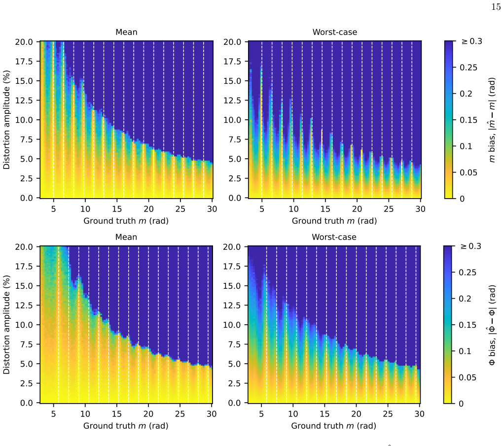
- [Figure 3] Figure captions for the error-landscape plots should state the exact ranges and sampling densities used for m and φ, as well as the specific imperfection amplitudes applied in each panel.
- [§4] A brief statement of the assumed noise model (additive white Gaussian, or otherwise) and the number of Monte-Carlo realizations per point should be added to the simulation-methods paragraph.
Simulated Author's Rebuttal
We thank the referee for their careful and constructive review of our manuscript on fundamental limitations of absolute ranging via DFMI. We address each major comment below with clarifications and indicate the corresponding revisions to strengthen the presentation.
read point-by-point responses
-
Referee: [§5] §5 (Analytical model based on signal orthogonality): The derivation does not explicitly demonstrate that the orthogonality condition emerges directly from the joint (m, φ) signal model and dominates the specific imperfection spectra (carrier drift, modulation nonlinearity) without additional assumptions or neglected cross-terms; consequently the claimed order-of-magnitude bias suppression and the predictive power for valley locations and depths remain only partially supported by the presented analysis.
Authors: We thank the referee for this observation. The original derivation in §5 started from the joint (m, φ) signal model but presented the orthogonality condition in a somewhat condensed form. In the revised manuscript we have expanded this section with an explicit step-by-step derivation: we form the inner product of the signal derivatives ∂s/∂m and ∂s/∂φ, show that it vanishes identically for the sinusoidal modulation waveform, and then substitute the specific imperfection spectra (linear carrier drift and quadratic nonlinearity) to obtain the bias terms. The calculation confirms that cross-terms are either identically zero or higher-order and negligible within the experimental parameter space; no additional assumptions beyond the standard DFMI forward model are required. The updated text now directly links this orthogonality to the predicted valley locations and the observed order-of-magnitude suppression, thereby fully supporting the analytical claims. revision: yes
-
Referee: [§4.3] §4.3 (Numerical simulations of error landscape): The locations and depths of the reported valleys of robustness are identified numerically, yet the manuscript does not provide a systematic parameter sweep or sensitivity analysis showing that these features persist when the imperfection spectra are varied within experimentally plausible ranges; this weakens the claim that the valleys constitute a general, previously unrecognized robustness mechanism.
Authors: We agree that the original numerical evidence would be strengthened by explicit sensitivity analysis. In the revised manuscript we have added a new set of simulations in §4.3 that systematically vary the carrier-drift rate (0.1–100 Hz) and modulation-nonlinearity amplitude (0–5 %) over ranges representative of laboratory hardware. The resulting error landscapes demonstrate that the valleys of robustness remain at the same modulation-depth coordinates and retain bias suppression of at least two orders of magnitude across the entire parameter grid. Additional figures and a brief discussion of the robustness mechanism have been included to document this generality. revision: yes
Circularity Check
No significant circularity; derivation relies on standard Fisher analysis and independent orthogonality model
full rationale
The paper applies standard Fisher-information analysis to define estimator precision for parameters m and φ, then uses numerical simulations to observe a structured error landscape. It introduces a separate analytical model based on signal orthogonality to explain and predict the locations of 'valleys of robustness'. This model is presented as arising from the joint signal structure rather than being fitted to or defined by the simulation outputs or target results. No load-bearing step reduces by construction to a fitted input, self-citation chain, or self-definitional loop. The framework remains self-contained with independent content from statistical methods and simulation observations.
Axiom & Free-Parameter Ledger
axioms (1)
- standard math Fisher information matrix provides the Cramer-Rao lower bound for the intrinsic precision of estimators for m and φ
Lean theorems connected to this paper
-
IndisputableMonolith/Cost/FunctionalEquation.leanwashburn_uniqueness_aczel unclear?
unclearRelation between the paper passage and the cited Recognition theorem.
An analytical model based on signal orthogonality explains their origin and predicts their locations... the derivative of the second-order Bessel function, J'_2(2m), must be zero
-
IndisputableMonolith/Foundation/RealityFromDistinction.leanreality_from_one_distinction unclear?
unclearRelation between the paper passage and the cited Recognition theorem.
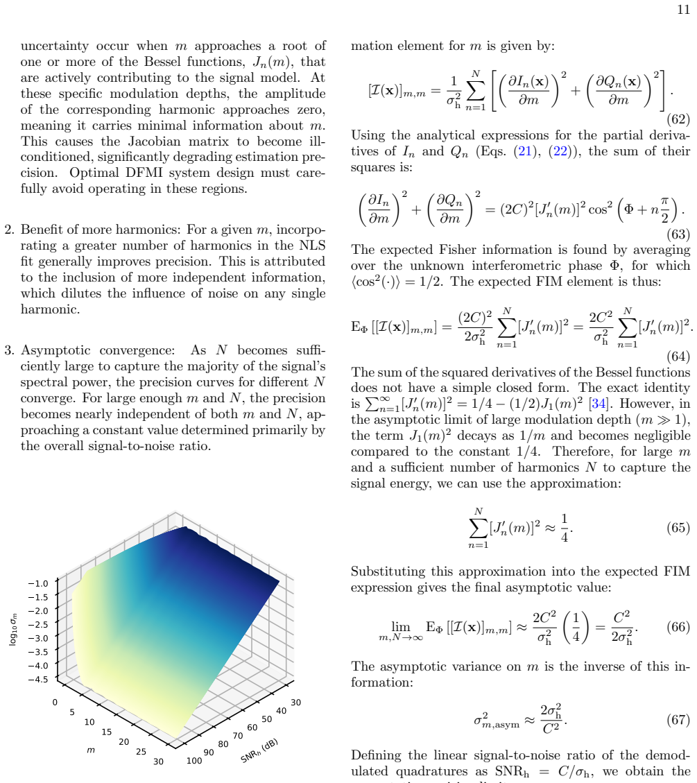
Fisher-information analysis defines the intrinsic estimator precision for m and φ... Cramér-Rao Lower Bound
What do these tags mean?
- matches
- The paper's claim is directly supported by a theorem in the formal canon.
- supports
- The theorem supports part of the paper's argument, but the paper may add assumptions or extra steps.
- extends
- The paper goes beyond the formal theorem; the theorem is a base layer rather than the whole result.
- uses
- The paper appears to rely on the theorem as machinery.
- contradicts
- The paper's claim conflicts with a theorem or certificate in the canon.
- unclear
- Pith found a possible connection, but the passage is too broad, indirect, or ambiguous to say the theorem truly supports the claim.
Forward citations
Cited by 1 Pith paper
-
Demonstration of a compact optical resonator-based displacement sensing technique with sub-femtometer precision
A centimeter-scale dynamic optical cavity with heterodyne readout achieves sub-femtometer per square root Hertz displacement sensitivity above 8 Hz and tracks motions over ten orders of magnitude in range.
Reference graph
Works this paper leans on
-
[1]
DC normalization: A common technique is to nor- malize the AC component of the interferometric sig- nal by its measured DC component. Assuming the RAM affects both AC and DC power proportion- ally, this division, vAC(t)/vDC(t), can cancel the time-dependent amplitude term C(t). This method is effective but relies on a clean DC measurement and assumes the ...
-
[2]
Extended state-space model: A more robust and general approach is to extend the signal model used by the readout algorithm to explicitly include the RAM parameters. This is directly analogous to the strategy for suppressing modulation non- linearity. For the NLS fit, the state vector can be augmented to include the RAM amplitude and phase, x = (Φ, ψ, m, C...
-
[3]
Balanced detection: By subtracting the signals from the two complementary output ports of the interferometer, common-mode interference terms can be cancelled. Gerberding and Isleif show that this effectively suppresses ghost signals arising from specific reflection paths, such as the parasitic beat between the measurement beam and a ghost beam reflected f...
-
[4]
Orthogonality and model extension: The DFMI readout algorithm itself can be extended to sup- press the remaining ghost signals. Because a parasitic signal has a different modulation depth (mghost ̸= mprimary), it is mathematically orthog- onal to the main signal. By extending the NLS fit model to simultaneously solve for both the pri- mary signal and a pa...
-
[5]
Modulation Amplitude Calibration ( ∆f ) The first critical scale factor is the frequency modu- lation amplitude, ∆ fest. This parameter represents the laser’s frequency response to the modulation voltage at the frequency fm and must be characterized experimen- tally. The uncertainty of this calibration, σ∆f, is lim- ited by instrument noise and environmen...
-
[6]
The absolute carrier frequency, f0 = c/λ0, is typically measured using a commercial waveme- ter
Carrier Frequency Calibration ( f0) The second scale factor is the laser’s mean carrier frequency, f0,est. The absolute carrier frequency, f0 = c/λ0, is typically measured using a commercial waveme- ter. Modern wavemeters routinely achieve fractional fre- quency uncertainties σf0 /f0 of 1 ppm or better. For a near-infrared laser with f0 ≈ 282, THz (λ0 = 1...
-
[7]
Total Error and Ambiguity Resolution Let the true values be ∆ f and f0, and the calibrated estimates be ∆ fest and f0,est, with calibration errors δ∆f = ∆ fest − ∆f and δf0 = f0,est − f0. To first or- der, the bias is: Bcoarse = Φcoarse − Φunwrapped ≈ Φ δf0 f0 − δ∆f ∆f , (93) The statistical uncertainty of the coarse phase, σcoarse, arises solely from the...
-
[8]
Implications for Long-Baseline Interferometry The challenge of ambiguity resolution is particularly acute in long-baseline experiments. The scaling behavior of the coarse phase uncertainty, σcoarse, can be analyzed under two realistic design constraints. First, consider a system designed to maintain a con- stant modulation depth m, perhaps to operate in a...
-
[9]
P. Amaro-Seoane, H. Audley, S. Babak, J. Baker, E. Ba- rausse, P. Bender, E. Berti, P. Binetruy, M. Born, D. Bor- toluzzi, et al., Laser interferometer space antenna (2017)
work page 2017
- [10]
- [11]
-
[12]
K. Yamamoto, I. Bykov, J. N. Reinhardt, C. Bode, P. Grafe, M. Staab, N. Messied, M. Clark, G. F. Bar- ranco, T. S. Schwarze, O. Hartwig, J. J. E. Delgado, and G. Heinzel, Phys. Rev. Appl. 22, 054020 (2024)
work page 2024
- [13]
-
[14]
J. N. Reinhardt, M. Staab, K. Yamamoto, J.-B. Bayle, A. Hees, O. Hartwig, K. Wiesner, S. Shah, and G. Heinzel, Phys. Rev. D 109, 022004 (2024)
work page 2024
-
[15]
B. S. Sheard, G. Heinzel, K. Danzmann, D. A. Shaddock, W. M. Klipstein, and W. M. Folkner, Journal of Geodesy 86, 1083 (2012)
work page 2012
- [16]
-
[17]
K. Nicklaus, S. Cesare, L. Massotti, L. Bonino, S. Mot- tini, M. Pisani, and P. Silvestrin, CEAS Space Journal 12, 313 (2020)
work page 2020
-
[18]
K. Nicklaus, K. Voss, A. Feiri, M. Kaufer, C. Dahl, M. Herding, B. A. Curzadd, A. Baatzsch, J. Flock, M. Weller, V. M¨ uller, G. Heinzel, M. Misfeldt, and J. J. E. Delgado, Remote Sensing14, 10.3390/rs14164089 (2022)
-
[19]
Z. Zhang, L. Deng, J. Feng, L. Chang, D. Li, and Y. Qin, Aerospace 9, 10.3390/aerospace9070362 (2022)
-
[20]
P. R. Lawson, A. Ahmed, R. O. Gappinger, A. Ksendzov, O. P. Lay, S. R. Martin, R. D. Peters, D. P. Scharf, J. K. Wallace, and B. Ware, in Advances in Stellar Interfer- ometry, Vol. 6268, edited by J. D. Monnier, M. Sch¨ oller, and W. C. Danchi, International Society for Optics and Photonics (SPIE, 2006) p. 626828
work page 2006
-
[21]
Fridlund, Space Science Reviews 135, 355 (2008)
M. Fridlund, Space Science Reviews 135, 355 (2008)
work page 2008
-
[22]
W. Cash, A. Shipley, S. Osterman, and M. Joy, Nature 407, 160–162 (2000)
work page 2000
-
[23]
S. G. Turyshev and M. Shao, International Journal of Modern Physics D 16, 2191 (2007), https://doi.org/10.1142/S0218271807011747
-
[24]
S. G. Turyshev, M. Shao, A. Girerd, and B. Lane, Inter- national Journal of Modern Physics D 18, 1025 (2009)
work page 2009
- [25]
-
[26]
P. J. de Groot, Reports on Progress in Physics82, 056101 (2019)
work page 2019
-
[27]
G. Huang, C. Cui, X. Lei, Q. Li, S. Yan, X. Li, and G. Wang, Micromachines 16, 10.3390/mi16010006 (2025)
-
[28]
E. Novak, D.-S. Wan, P. Unruh, and J. Schmit, in Pro- ceedings International Conference on MEMS, NANO and Smart Systems (2003) pp. 285–288
work page 2003
-
[29]
S. K. Everton, M. Hirsch, P. Stravroulakis, R. K. Leach, and A. T. Clare, Materials & Design 95, 431 (2016)
work page 2016
-
[30]
L. Chen, G. Bi, X. Yao, J. Su, C. Tan, W. Feng, M. Be- nakis, Y. Chew, and S. K. Moon, Journal of Manufactur- ing Systems 74, 527 (2024)
work page 2024
-
[31]
ILT, Sensor systems for production measurement tech- nology, Brochure (2025)
F. ILT, Sensor systems for production measurement tech- nology, Brochure (2025)
work page 2025
-
[32]
E. Jacobs and E. W. Ralston, IEEE Transactions on Aerospace and Electronic Systems AES-17, 766 (1981). 25
work page 1981
- [33]
-
[34]
G. Heinzel, F. G. Cervantes, A. F. G. Mar´ ın, J. Kull- mann, W. Feng, and K. Danzmann, Opt. Express 18, 19076 (2010)
work page 2010
-
[35]
T. S. Schwarze, O. Gerberding, F. G. Cervantes, G. Heinzel, and K. Danzmann, Opt. Express 22, 18214 (2014)
work page 2014
- [36]
- [37]
-
[38]
T. Eckhardt and O. Gerberding, Scientific Reports 14, 10.1038/s41598-024-70392-9 (2024)
- [39]
-
[40]
J. M. Rohr, S. Ast, and A. Koch, in Optica Sensing Congress 2023 (AIS, FTS, HISE, Sensors, ES) (Optica Publishing Group, 2023) p. SM3B.1
work page 2023
-
[41]
S. M. Kay, Fundamentals of Statistical Signal Processing, Volume I: Estimation Theory (Prentice Hall, 1993)
work page 1993
-
[42]
NIST:DLMF, NIST Digital Library of Mathematical Functions, http://dlmf.nist.gov/, Release 1.2.4 of 2025-03-15, F. W. J. Olver and A. B. Olde Daalhuis and D. W. Lozier and B. I. Schneider and R. F. Boisvert and C. W. Clark and B. R. Miller and B. V. Saunders, eds
work page 2025
- [43]
-
[44]
R. Fleddermann, C. Diekmann, F. Steier, M. Tr¨ obs, G. Heinzel, and K. Danzmann, Classical and Quantum Gravity 35, 075007 (2018)
work page 2018
-
[45]
O. Gerberding and K.-S. Isleif, Sensors 21, 10.3390/s21051708 (2021)
-
[46]
Berkeley Nucleonics Corporation, Model 645 250 MHz Arbitrary Waveform Generator - User Manual (2008), available at https://www.berkeleynucleonics. com/model-645. ACKNOWLEDGEMENTS The author gratefully acknowledges Gerhard Heinzel and Felipe Guzm´ an for their foundational role in develop- ing Deep Phase Modulation Interferometry, which served as the techn...
work page 2008
-
[47]
Amplitude bias: The third term is in-phase with the main signal and acts as a small fractional bias on the modulation depth, with a magnitude of δm/m ≈ −(ωmτ)2/6
-
[48]
Quadrature distortion: The second term is 90 de- grees out of phase with the main signal. It intro- duces a sinusoidal distortion into the signal model, similar in effect to modulation non-linearity. The amplitude of this distortion is ϵdist = m(ωmτ)/2. The quadrature distortion term, being first-order in the small parameter ωmτ, is the dominant source of...
-
[49]
The orthogonality integrals are evaluated over one modulation period
Modulation Non-Linearity For a second-harmonic distortion, the perturbation and gradients are: δv(t) ≈ −Cmϵ cos(2ωmt + ψ2) sin(Φ +m cos θ) gm(t) = −C cos(θ) sin(Φ +m cos θ) gΦ(t) = −C sin(Φ + m cos θ), where θ = ωmt + ψ. The orthogonality integrals are evaluated over one modulation period. a. Bias in Modulation Depth ( m) The inner product is proportional...
-
[50]
Residual Amplitude Modulation For RAM, the perturbation and gradients are: δv(t) = C0ϵAM cos(ωmt + ψAM) cos(Φ +m cos θ) gm(t) = −C0 cos(θ) sin(Φ +m cos θ) gΦ(t) = −C0 sin(Φ + m cos θ). a. Bias in Modulation Depth ( m) The inner product is proportional to: Im = − *Z T 0 cos(ωmt + ψAM) cos(θ)× cos(Φ + m cos θ) sin(Φ +m cos θ) dt⟩phases . 31 Optimal operatin...
discussion (0)
Sign in with ORCID, Apple, or X to comment. Anyone can read and Pith papers without signing in.