Two Tunable Gini-Type Measures with U-Statistic Estimation: Theory, Simulation, and an Empirical Application to GDP per Capita in the Americas

Helton Saulo; Roberto Vila

arxiv: 2508.02965 · v2 · submitted 2025-08-05 · 📊 stat.ME

Two Tunable Gini-Type Measures with U-Statistic Estimation: Theory, Simulation, and an Empirical Application to GDP per Capita in the Americas

Roberto Vila , Helton Saulo This is my paper

Pith reviewed 2026-05-19 01:27 UTC · model grok-4.3

classification 📊 stat.ME

keywords inequality measuresGini coefficientU-statisticsasymptotic normalitytunable indicesGDP per capitaMonte Carlo simulationconsistency

0 comments

The pith

Two new families of inequality measures recover the Gini coefficient at large tuning values and admit closed-form U-statistic estimators with proven consistency.

A machine-rendered reading of the paper's core claim, the machinery that carries it, and where it could break.

The paper defines two parametric families of inequality indices, G_p for p greater than 1 and H_q for q positive, that let the user control how strongly large pairwise gaps affect the final number. Both families are constructed so that they approach the ordinary Gini coefficient when the tuning parameter is sent to infinity. Closed-form estimators based on U-statistics are supplied for each index, and these estimators are shown to be strongly consistent and asymptotically normal as long as the underlying distribution satisfies only mild moment conditions. A simulation study checks how the estimators behave in finite samples for different choices of n, p and q, while an application to GDP-per-capita data from the Americas illustrates how the tuning parameters change the measured level of inequality.

Core claim

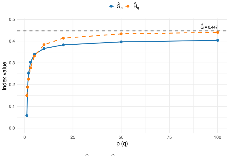
The paper introduces two families of inequality measures G_p and H_q that converge to the classical Gini coefficient as p and q tend to infinity. For each family the authors derive explicit U-statistic plug-in estimators and establish strong consistency together with asymptotic normality under mild moment conditions on the distribution.

What carries the argument

The tunable indices G_p and H_q, which weight pairwise absolute differences by a power parameter that can be adjusted to emphasize or dampen the contribution of extreme disparities.

If this is right

Analysts can compute the new measures directly from a sample without iterative numerical methods.
Asymptotic normality supplies approximate confidence intervals for the inequality level at any fixed tuning value.
Varying the parameters p or q produces a continuous range of inequality readings that all collapse to the same Gini limit.
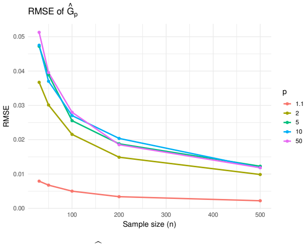
The Monte Carlo results indicate that the estimators remain reliable for moderate sample sizes once the tuning parameters are not chosen extremely large.

Where Pith is reading between the lines

These are editorial extensions of the paper, not claims the author makes directly.

Policy analysts could use the tuning parameters to perform sensitivity checks that reflect different societal priorities on top-end versus bottom-end disparities.
The framework could be extended to other classical inequality indices by replacing the absolute-difference kernel with a different symmetric kernel while preserving the U-statistic estimation route.
In cross-country comparisons, reporting a short table of values for several p or q choices would let readers see how sensitive the ranking of nations is to the chosen emphasis on large gaps.

Load-bearing premise

The data must satisfy mild moment conditions so that the asymptotic consistency and normality of the U-statistic estimators continue to hold.

What would settle it

Draw repeated large samples from a distribution whose second moment is infinite; the claimed asymptotic normality of the estimators would then fail to appear.

Figures

Figures reproduced from arXiv: 2508.02965 by Helton Saulo, Roberto Vila.

**Figure 1.** Figure 1: Behavior of the estimators Gbp and Hbq defined in equations (3) and (4), respectively, as functions of p (q). The dashed line represents the classical Gini estimator Gb. Estimates were computed using a sample of size n = 50 drawn from a Gamma distribution with shape 1.5 and scale 2.5. To fully understand the role of p and q on the computation of Gbp and Hbq, we plot the values of p and q against T(p) ≡ log… view at source ↗

**Figure 2.** Figure 2: Curves of T(p) = log 1 + p X2−X1 + log 1 + p X1−X2 for various pairs (X1, X2). 0 25 50 75 1 2 3 4 5 6 7 8 9 10 q K(q) (X1 ,X2 ) (10,100) (10,20) (10,50) (2,100) (2,20) (2,50) [PITH_FULL_IMAGE:figures/full_fig_p005_2.png] view at source ↗

**Figure 3.** Figure 3: Curves of K(q) = X q 1 +X q 2 2 1/q − X −q 1 +X −q 2 2 −1/q for several pairs (X1, X2). is a U-statistic (Hoeffding, 1948) and g(Xi , Xj ) ≡ log 1 + p Xj−Xi + log 1 + p Xi−Xj − 2 log(2) log(p) . (6) If E |g(X1, X2)| < ∞, then, by strong law of large numbers for U-Statistics (Lee, 1990; Henze, 2024), Un a.s. −→ E [g(X1, X2)] , as n → ∞, with a.s. −→ meaning almost sure convergence. Since X a.s. −→ µ, … view at source ↗

**Figure 4.** Figure 4: MARE of Gbp for varying sample sizes and values of p. 0.04 0.08 0.12 100 200 300 400 500 Sample size (n) MARE q 1.1 2 5 10 50 MARE of H^ q [PITH_FULL_IMAGE:figures/full_fig_p010_4.png] view at source ↗

**Figure 5.** Figure 5: MARE of Hbq for varying sample sizes and values of q. 10 [PITH_FULL_IMAGE:figures/full_fig_p010_5.png] view at source ↗

**Figure 6.** Figure 6: RMSE of Gbp for varying sample sizes and values of p. 0.01 0.02 0.03 0.04 0.05 100 200 300 400 500 Sample size (n) RMSE q 1.1 2 5 10 50 RMSE of H^ q [PITH_FULL_IMAGE:figures/full_fig_p011_6.png] view at source ↗

**Figure 7.** Figure 7: RMSE of Hbq for varying sample sizes and values of q. 8 Application In this section, we illustrate the proposed income inequality measures using a data set on gross domestic product (GDP) per capita for all countries and territories in the Americas in 2023. The raw data (in international dollars at 2021 prices) were downloaded from Our World in Data https://ourworldindata.org/grapher/gdp-per-capita-worldba… view at source ↗

**Figure 8.** Figure 8: Diagnostic plots for the gamma distribution fitted to GDP pe [PITH_FULL_IMAGE:figures/full_fig_p012_8.png] view at source ↗

**Figure 9.** Figure 9: Estimated values of Gbp and Hbq for parameters p, q ∈ {1.1, 1.5, 2, 3, 5, 10}. The dashed line indicates the classical Gini coefficient Gb. 9 Concluding remarks In this paper we have introduced two flexible inequality measures, Gp and Hq, which generalize the classical Gini coefficient. By deriving closed-form U-statistic estimators for each index, we established strong consistency and asymptotic normality… view at source ↗

read the original abstract

We introduce two families of inequality measures, $G_p$ and $H_q$, that converge to the classical Gini coefficient as $p,q\to\infty$. The tuning parameters $p>1$ and $q>0$ regulate the influence of disparities between observations. For each index we derive closed-form $U$-statistic plug-in estimators and establish strong consistency and asymptotic normality under mild moment conditions. A Monte Carlo study assesses finite-sample behavior across $(n,p,q)$, and an empirical illustration with GDP per capita in the Americas shows how the tuning parameters influence the measure of inequality.

Editorial analysis

A structured set of objections, weighed in public.

Desk editor's note, referee report, simulated authors' rebuttal, and a circularity audit. Tearing a paper down is the easy half of reading it; the pith above is the substance, this is the friction.

Desk Editor's Note private letter to a colleague

The paper gives two parametric Gini-type families with closed-form U-statistic estimators and limit behavior, but the asymptotic normality rests on moment conditions that may fail for heavy-tailed GDP data.

read the letter

Hey colleague, the main thing here is that the authors introduce two tunable families of inequality measures, G_p and H_q, that converge to the standard Gini as the parameters grow large, and they supply explicit U-statistic estimators plus consistency and normality results under mild moment conditions. They also run Monte Carlo checks and apply the measures to GDP per capita across the Americas to show how the tuning affects the numbers. What is actually new is the specific parametric forms that let the user control the influence of larger disparities, together with the closed-form estimators that avoid more complicated computation. That combination is a modest but direct extension of the existing Gini literature, and the simulation and application sections give concrete illustrations of how the indices behave in practice. The soft spot is the asymptotic theory. Standard U-statistic central limit theorems require a finite second moment on the kernel, and the stress-test concern is reasonable: GDP per capita often follows heavy-tailed distributions, and the tuning parameters can make the kernel even heavier in the tails. The paper labels the conditions mild but does not appear to verify them on the data or discuss when they hold, which leaves the reliability of the normality result open for the empirical part. This work is aimed at applied statisticians and economists who measure inequality and want flexible alternatives for sensitivity checks. A reader looking for practical extensions of classical indices with ready estimators would get value from it. I would bring it to a reading group to talk through the moment conditions. It deserves a serious referee because the core construction is clear and the estimators are explicit, even if the application needs more scrutiny on the asymptotics. Recommendation: send it for peer review.

Referee Report

2 major / 2 minor

Summary. The manuscript introduces two families of tunable inequality measures G_p (p>1) and H_q (q>0) that converge to the classical Gini coefficient as p,q → ∞. For each, the authors derive closed-form U-statistic plug-in estimators and establish strong consistency plus asymptotic normality under mild moment conditions. A Monte Carlo study examines finite-sample behavior over ranges of n, p, and q, and an empirical illustration applies the measures to GDP per capita across countries in the Americas to show the effect of the tuning parameters on measured inequality.

Significance. If the derivations and moment conditions hold, the work supplies a flexible, theoretically grounded extension of the Gini index with explicit estimators and limiting distributions. The U-statistic construction and convergence property are strengths that could support sensitivity analyses in inequality studies. The Monte Carlo design and real-data example provide practical grounding, though the value depends on whether the asymptotics apply to the heavy-tailed distributions typical in such applications.

major comments (2)

[§4, Theorem 3] §4 (Asymptotic Properties), Theorem 3 and the statement of 'mild moment conditions': Asymptotic normality of the U-statistic estimator requires E[h(X_1,X_2)^2] < ∞ for the symmetric kernel h. The paper should explicitly state the moment requirements on the underlying distribution in terms of p (or q) and verify that they are satisfied for the GDP per capita data, whose tails are typically Pareto with index near 2–3. If the kernel involves terms such as |X_i − X_j|^p, the second-moment condition on h may demand higher moments than the label 'mild' suggests, directly affecting the reliability of the asymptotic inference claimed for the empirical illustration.
[§6] §6 (Empirical Application): The data description does not specify how extreme observations or potential outliers are handled, nor does it report whether the moment conditions required by the asymptotic theorems are checked for the sample. Because the central claim includes reliable estimation and inference for real data, this omission weakens the link between the theoretical results and the reported findings on how p and q affect measured inequality.

minor comments (2)

[§1] The introduction would benefit from a short table comparing G_p and H_q to the classical Gini and to other tunable indices (e.g., generalized entropy) to clarify the novelty.
[§5] In the Monte Carlo section, the reported bias and variance tables should include the exact sample sizes and parameter grids used so that readers can replicate the finite-sample assessment.

Simulated Author's Rebuttal

2 responses · 0 unresolved

We are grateful to the referee for their constructive comments on our paper. These suggestions will help clarify the theoretical foundations and strengthen the connection to the empirical results. We address the major comments below and outline the revisions we intend to implement.

read point-by-point responses

Referee: [§4, Theorem 3] §4 (Asymptotic Properties), Theorem 3 and the statement of 'mild moment conditions': Asymptotic normality of the U-statistic estimator requires E[h(X_1,X_2)^2] < ∞ for the symmetric kernel h. The paper should explicitly state the moment requirements on the underlying distribution in terms of p (or q) and verify that they are satisfied for the GDP per capita data, whose tails are typically Pareto with index near 2–3. If the kernel involves terms such as |X_i − X_j|^p, the second-moment condition on h may demand higher moments than the label 'mild' suggests, directly affecting the reliability of the asymptotic inference claimed for the empirical illustration.

Authors: We agree with the referee that the moment conditions warrant more explicit statement. In the revised version, we will expand the discussion in Section 4 to derive and state the precise moment requirements for asymptotic normality of the estimators of G_p and H_q. Specifically, for the kernel involving |X_i - X_j|^p, this requires the underlying random variable to have a finite moment of order 2p (for positive support). We will also include a brief verification or discussion for the GDP per capita data in the empirical section, noting the sample moments or the range of p and q for which the conditions are plausibly met given typical tail indices of 2-3. This addresses the concern about reliability of asymptotic inference. revision: yes
Referee: [§6] §6 (Empirical Application): The data description does not specify how extreme observations or potential outliers are handled, nor does it report whether the moment conditions required by the asymptotic theorems are checked for the sample. Because the central claim includes reliable estimation and inference for real data, this omission weakens the link between the theoretical results and the reported findings on how p and q affect measured inequality.

Authors: We acknowledge this gap in the current manuscript. In the revision, we will enhance Section 6 by adding details on data preprocessing, including any handling of extreme observations or outliers (e.g., winsorizing or log-transformation if applied). Additionally, we will report checks or discussions regarding the satisfaction of the moment conditions for the chosen tuning parameters. These additions will better connect the theoretical results to the empirical findings. revision: yes

Circularity Check

0 steps flagged

No significant circularity; standard U-statistic theory applied to newly defined kernels

full rationale

The paper defines the tunable measures G_p and H_q directly as functionals of the distribution (converging to Gini as p,q→∞), expresses each as an expectation of a symmetric kernel, and obtains the plug-in estimator as the corresponding U-statistic. Strong consistency and asymptotic normality then follow from the classical Hoeffding or Serfling theorems once the kernel satisfies the stated moment conditions. These steps invoke only external, non-self-referential results on U-statistics; no parameter is fitted to the target data and then relabeled a prediction, no uniqueness theorem is imported from the authors' prior work, and the derivation does not reduce to a tautology or self-citation chain. The empirical GDP illustration is presented separately as an application, not as the source of the asymptotic claims.

Axiom & Free-Parameter Ledger

2 free parameters · 1 axioms · 0 invented entities

The central claim rests on the direct definition of the new G_p and H_q families plus standard U-statistic theory; the tuning parameters are user-chosen rather than data-fitted, and no new physical or mathematical entities are postulated.

free parameters (2)

p
Tuning parameter greater than 1 that controls the weight given to disparities in the G_p family.
q
Tuning parameter greater than 0 that controls the weight given to disparities in the H_q family.

axioms (1)

domain assumption Mild moment conditions on the underlying random variables
Invoked to guarantee strong consistency and asymptotic normality of the U-statistic estimators.

pith-pipeline@v0.9.0 · 5630 in / 1338 out tokens · 45104 ms · 2026-05-19T01:27:14.888663+00:00 · methodology

discussion (0)

Reference graph

Works this paper leans on

12 extracted references · 12 canonical work pages

[1]

H., Zou, H., and Yao, H

Baydil, B., de la Pe˜ na, V. H., Zou, H., and Yao, H. (2025). Unbiased es timation of the gini coeﬃcient. Statistics and Probability Letters

work page 2025
[2]

and Weiner, J

Damgaard, C. and Weiner, J. (2000). Describing inequality in plant siz e or fecundity. Ecology, 81:1139–1142

work page 2000
[3]

Deltas, G. (2003). The small-sample bias of the gini coeﬃcient: Resu lts and implications for empirical research. Review of Economics and Statistics , 85:226–234

work page 2003
[4]

M., Ruiz-G´ andara, A., Ortega-Irizo, F

Gavilan-Ruiz, J. M., Ruiz-G´ andara, A., Ortega-Irizo, F. J., and Gon zalez-Abril, L. (2024). Some notes on the gini index and new inequality measures: The nth gini inde x. Stats, 7:1354–1365

work page 2024
[5]

Gini, C. (1936). On the measure of concentration with special refe rence to income and statistics. Colorado College Publication, General Series No. 208 , pages 73–79

work page 1936
[6]

Henze, N. (2024). Asymptotic Stochastics: An Introduction with a View toward s Statistics. Springer

work page 2024
[7]

Hoeﬀding, W

Berlin, Heidelberg. Hoeﬀding, W. (1948). A class of statistics with asymptotically norma l distribution. Annals of Mathematical Statistics, 19:293–325

work page 1948
[8]

Kharazmi, E., Bordbar, N., and Bordbar, S. (2023). Distribution of nursing workforce in the world using gini coeﬃcient. BMC Nursing , 22:151

work page 2023
[9]

Lee, A. J. (1990). U-Statistics. Marcel Dekker, New York

work page 1990
[10]

Sun, T., Zhang, H., Wang, Y., Meng, X., and Wang, C. (2010). The app lication of environmental gini coeﬃcient (egc) in allocating wastewater discharge permit: The case study of watershed total mass control in tianjin, china. Resources, Conservation and Recycling , 54(9):601–608

work page 2010
[11]

and Saulo, H

Vila, R. and Saulo, H. (2025). The mth gini index estimator: Unbiasedness for gamma populations. Manuscript submitted for publication. Preprint

work page 2025
[12]

Yao, S. (1999). On the decomposition of gini coeﬃcients by populat ion class and income source: a spreadsheet approach and application. Applied Economics, 31(10):1249–1264. 14

work page 1999

[1] [1]

H., Zou, H., and Yao, H

Baydil, B., de la Pe˜ na, V. H., Zou, H., and Yao, H. (2025). Unbiased es timation of the gini coeﬃcient. Statistics and Probability Letters

work page 2025

[2] [2]

and Weiner, J

Damgaard, C. and Weiner, J. (2000). Describing inequality in plant siz e or fecundity. Ecology, 81:1139–1142

work page 2000

[3] [3]

Deltas, G. (2003). The small-sample bias of the gini coeﬃcient: Resu lts and implications for empirical research. Review of Economics and Statistics , 85:226–234

work page 2003

[4] [4]

M., Ruiz-G´ andara, A., Ortega-Irizo, F

Gavilan-Ruiz, J. M., Ruiz-G´ andara, A., Ortega-Irizo, F. J., and Gon zalez-Abril, L. (2024). Some notes on the gini index and new inequality measures: The nth gini inde x. Stats, 7:1354–1365

work page 2024

[5] [5]

Gini, C. (1936). On the measure of concentration with special refe rence to income and statistics. Colorado College Publication, General Series No. 208 , pages 73–79

work page 1936

[6] [6]

Henze, N. (2024). Asymptotic Stochastics: An Introduction with a View toward s Statistics. Springer

work page 2024

[7] [7]

Hoeﬀding, W

Berlin, Heidelberg. Hoeﬀding, W. (1948). A class of statistics with asymptotically norma l distribution. Annals of Mathematical Statistics, 19:293–325

work page 1948

[8] [8]

Kharazmi, E., Bordbar, N., and Bordbar, S. (2023). Distribution of nursing workforce in the world using gini coeﬃcient. BMC Nursing , 22:151

work page 2023

[9] [9]

Lee, A. J. (1990). U-Statistics. Marcel Dekker, New York

work page 1990

[10] [10]

Sun, T., Zhang, H., Wang, Y., Meng, X., and Wang, C. (2010). The app lication of environmental gini coeﬃcient (egc) in allocating wastewater discharge permit: The case study of watershed total mass control in tianjin, china. Resources, Conservation and Recycling , 54(9):601–608

work page 2010

[11] [11]

and Saulo, H

Vila, R. and Saulo, H. (2025). The mth gini index estimator: Unbiasedness for gamma populations. Manuscript submitted for publication. Preprint

work page 2025

[12] [12]

Yao, S. (1999). On the decomposition of gini coeﬃcients by populat ion class and income source: a spreadsheet approach and application. Applied Economics, 31(10):1249–1264. 14

work page 1999