REVIEW 5 major objections 4 minor 1 cited by
Marketron Through the Looking Glass: From Equity Dynamics to Option Pricing in Incomplete Markets
T0 review · 5 major / 4 minor · reviewed 2026-08-05 · deepseek-v4-flash
Pith's one-line read The Marketron model can be calibrated to option prices through a fast utility-indifference pricing scheme, but the same calibration fails to reproduce realized equity volatility.
desk verdict Interesting numerical machinery, but the pricer outputs no-arbitrage-violating prices, so the calibration claim doesn't stand. read the letter →
The pith
A machine-rendered reading of the paper's core claim, the machinery that carries it, and where it could break.
The reading
What carries the argument
The central object is the 3D Marketron diffusion $(x, y, \theta)$ with the marketron potential $V(x,y)$ and its nonlinear drift $\mu_x$. The argument's load-bearing engine is a four-step numerical chain: a generalized Duhamel's principle converts the quadratic-nonlinearity HJB PDE into a nonlinear Volterra integral equation of the second kind with a known 3D Gaussian Green's function kernel; Gaussian RBF collocation evaluates all integrals in closed form; Strang splitting decomposes the 3D problem into 1D steps; and the Cole-Hopf transformation turns the nonlinear steps into linear PDEs, so each time step requires only linear solves with multiple right-hand sides, one per strike. The compani
What would settle it
Compute the same SPY option prices as in Tables 3 and 5 using the original $f(\theta)$ and $V'_M(x)$ of Eqs. (2)–(3) with a fine-grid finite-difference or Monte Carlo solver of the same HJB/indifference-pricing problem, and check whether prices differ by more than the reported 3–8% calibration residual; if they do, the calibrated parameters are artifacts of the substitute functions. A cheaper check: rerun the RBF scheme with, say, $40\times10\times10$ points or a better-conditioned basis and see whether calibrated parameters and option prices move materially.
Extended reading notes
Core claim
On the paper's own terms, the discovery is a complete pipeline from Marketron dynamics to market option prices. With exponential utility, indifference pricing yields a certainty-equivalent PDE whose solution gives option prices as log-ratios of two value functions; the tradable-factor market price of risk collapses to $(\mu_x - r)/\sigma$, the complete-market form, but inherits state dependence through the nonlinear drift $\mu_x$. The PDE is solved by converting it to a nonlinear Volterra integral equation of the second kind via a generalized Duhamel's principle, discretizing with Gaussian RBFs that make all matrix elements closed-form, and using Strang splitting so that Cole-Hopf transforms
Load-bearing premise
The calibration stands or falls on the assumption that the analytically convenient substitutes for the model's signal function $f(\theta)$ and price-impact derivative $V'_M(x)$, used with a $20\times5\times5$ RBF grid whose matrix condition number is about $10^{19}$, produce option prices close enough to the original Marketron dynamics that the fitted parameters describe the intended model.
Editorial extensions
If this is right
- If the calibration pipeline is correct, option prices under the Marketron model become computable in seconds on standard hardware, with all strikes at a maturity handled in a single linear solve.
- The market price of risk being $(\mu_x - r)/\sigma$ with state-dependent $\mu_x$ implies the model generates a time-varying, path-dependent equity risk premium from a constant-volatility diffusion.
- Calibrating to option data under the risk-minimal measure does not automatically transfer to real-measure equity dynamics: the fitted model overstates historical volatility, so pricing and statistical calibration need separate targets or a genuinely joint estimator.
- The reported Hurst exponents near 0.3 from an option-calibrated pure diffusion suggest rough-path-like behavior can emerge from nonlinear drift alone, without fractional Brownian motion or jumps.
- The explicit admission that joint calibration fails means models with memory drift and uncorrelated noises are insufficient for the SPX/option consistency problem, supporting the need for correlation or path-dependent local volatility.
- The numerical scheme's efficiency means that adding more strikes to a calibration is nearly free, so smile calibration within this framework is limited mainly by model flexibility rather than by computational cost.
Reading between the lines
- Editorial extension: because the solvable scheme replaces $f(\theta)$ and $V'_M(x)$ by qualitatively similar substitutes (Appendix B), the calibrated parameters describe a tractable cousin of the Marketron model; pricing the original functions with a fine-grid independent solver is a direct robustness test the paper does not run.
- Editorial extension: the state-dependent market price of risk formula creates a testable bridge between the model and data: simulated MPR time series could be compared with option-implied equity risk premia over bull/bear regimes, where the paper already notes the sign can flip.
- Editorial extension: the single-maturity, constant-parameter calibration used here cannot identify time-dependent model functions; extending the Volterra/RBF machinery to multi-maturity calibration would require time-dependent Green's functions or forward PDEs, a natural next step given the paper tried multi-maturity calibration and deemed it insufficiently accurate.
- Editorial extension: if the joint-calibration failure is indeed due to uncorrelated Brownian motions, adding a mixed-derivative term to the splitting (as the paper suggests) is a cheap, falsifiable modification; the 2017 episode of low realized and high implied volatility is a sharp test case for whether correlation alone closes the volatility gap.
Signed reviews
Editorial analysis
A structured set of objections, weighed in public.
Referee Report
Summary. The paper extends the Marketron model of Halperin and Itkin to option pricing in an incomplete market. It derives an exponential-utility indifference pricing framework, obtains a nonlinear HJB PDE for the certainty-equivalent option price, and proposes two numerical solvers: a Volterra-integral/RBF method and a Strang-splitting method with Cole-Hopf transformations. It then calibrates the resulting pricer to a snapshot of SPX option prices, reports calibrated parameters for two maturities, computes simulation-based moments of underlying log-returns, and derives a market price of risk. The central claims are that the framework 'solves the problem of calibration of the Marketron model to market option data' (Section 6) and that the tradable-factor market price of risk equals (mu_x - r)/sigma in Eq. (37).
Significance. If the numerical machinery and model calibration were sound, the paper would contribute a useful computational toolkit for utility-based pricing in a non-affine, three-dimensional incomplete-market model. The closed-form RBF/Green's-function integrals in Appendix A and the Strang-splitting/Cole-Hopf decomposition are elegant ideas, and the authors are transparent about the model's failure to jointly match option and equity time-series moments. However, the paper's central empirical claims are not supported by the evidence it presents. The option tables violate basic no-arbitrage inequalities, the market price of risk equation is internally inconsistent with the preceding derivation, and the tractable pricing model replaces key Marketron functions with qualitatively similar substitutes without validating the effect on prices. These issues are load-bearing for the calibration claim, so the significance of the paper as a contribution to option pricing is currently not established.
major comments (5)
- [§3.2, Eqs. (36)–(37)] Equation (37) does not follow from Eq. (36) and Eq. (21) given the definition of \bar{\mu}_x in Eq. (7). With \bar{\mu}_x = \mu_x + \frac12\sigma^2 - r, substituting h^V - \partial_s C = \bar{\mu}_x/(\gamma s \sigma^2) into Eq. (36) yields \lambda^{(x)} = \bar{\mu}_x/\sigma = (\mu_x + \frac12\sigma^2 - r)/\sigma, not (\mu_x - r)/\sigma. This is not a minor typo: Section 5.2.4 and Figures 4–6 report market prices of risk computed from Eq. (37), so all reported MPR values are shifted by \sigma/2.
- [§4.1, Table 3] The option prices in Table 3 violate static no-arbitrage constraints for European calls. For fixed S = 950, C(K=975) = 116.61 while C(K=985) = 124.29, so the price increases in strike. For fixed S = 985, C(K=975) = 110.68 while C(K=985) = 127.51. For fixed K = 950, C(S=950) = 126.33 while C(S=975) = 122.18, so the price decreases in spot. These violations are tens of dollars, not round-off noise. A pricer that violates call-spread monotonicity and spot monotonicity is not a valid pricing map, and calibrating through this pricer does not establish parameters of the Marketron model.
- [Appendix B, Eqs. (B.2) and (B.10)] To obtain closed-form integrals, the paper replaces V'_M(x) with the erfc-based regularizer R_2(x) and f(θ) with the normal-CDF approximation f_1(θ). The justification is visual similarity in Figures 7–8. No quantitative test is provided that option prices under the substitutes approximate prices under the original functions. Appendix B.1 explicitly says the original integral 'cannot be taken in closed form' and that the function definition is changed. As a result, the calibrated parameters in Tables 5–6 describe a modified model, not the original Marketron dynamics of Eqs. (1)–(3). This directly undermines the paper's central calibration claim.
- [§4.1, RBF discretization] The numerical scheme is used for the calibration but is not validated to the required accuracy. The paper uses N_x = 20, N_y = 5, N_θ = 5 collocation points, states that the Gaussian RBF matrix has condition number approximately 10^19, and notes that 'even iterative solving methods produce larger errors.' No convergence study or comparison against a trusted PDE/Monte Carlo solver is reported. In the presence of the no-arbitrage violations in Table 3, the pricer cannot be considered reliable enough for the 5–8% calibration accuracy claimed in Section 5.2.2.
- [§5.2.2, §6] The paper's own reported results contradict the claim that it 'solves the problem of calibration of the Marketron model to market option data.' Section 5.2.2 reports relative calibration accuracy of about 8% for Calls and Puts and about 3% for Puts only. Section 6 explicitly states that the model 'fails to solve the joint calibration problem' and admits that the nonlinear constraints may exclude the true global minimum or overly restrict the solution domain. These admissions, combined with the invalid price tables and the unvalidated model substitutions, make the concluding claim unsupported.
minor comments (4)
- [§5.1, Eqs. (71)–(72)] The discussion first replaces f and h by linear functions of θ, then by cos(θ) and sin(θ) to keep Green's-function convolutions tractable. The relationship between these two reductions and the stated preference for monotone bounded functions is confusing and should be reorganized.
- [Appendix A, Eq. (A.14)] The notation 'J_i = ∫ J_i(ξ) ...' reuses the same symbol for the integral and the integrand, making the formula difficult to follow.
- [Appendix B, Eq. (B.15)] The definitions of a_+(σ_θ), α_{θ,1}, and β_{θ,1} mix a(σ) and a_+(σ) inconsistently; please check whether the intended variance scaling is that of Eq. (A.7) or a genuinely different one.
- [§5.2.4, Figures 4–6] The MPR figures would benefit from a statement of which formula was used (Eq. (36) versus Eq. (37)) and how the σ²/2 term is handled, given the inconsistency raised in the major comments.
Circularity Check
No significant circularity: the option-pricing derivation is self-contained and the calibration is a genuine inverse problem.
full rationale
The paper derives its pricing measure from the external indifference-pricing framework of Grasselli and Hurd (2007) and applies the HJB-to-Volterra/RBF pipeline to that PDE, rather than fitting the pricing formula to the target option prices. The Marketron SDEs are inherited from the authors' prior preprint, but they serve as the input model under study, not as a conclusion drawn from option data; citing one's own model is a normal modeling choice and does not make the new calibration circular. The calibrated parameters are obtained by least-squares optimization against option quotes, and the reported log-return statistics in Tables 7–9 are produced by Monte Carlo simulation of the calibrated SDEs, not by inverting the option fit. The paper explicitly concedes that the joint calibration problem is not solved and that calibration accuracy is only about 5–8%, which weakens the central claim but does not constitute a by-construction reduction. The replacement of V'_M and f by analytically tractable regularizers in Appendix B and the ill-conditioned RBF matrices are numerical-fidelity caveats, not circularity. No step was found where an equation is defined in terms of its target, a fitted parameter is renamed a prediction, or a load-bearing premise rests solely on a self-citation.
Assumptions & free parameters
free parameters (14)
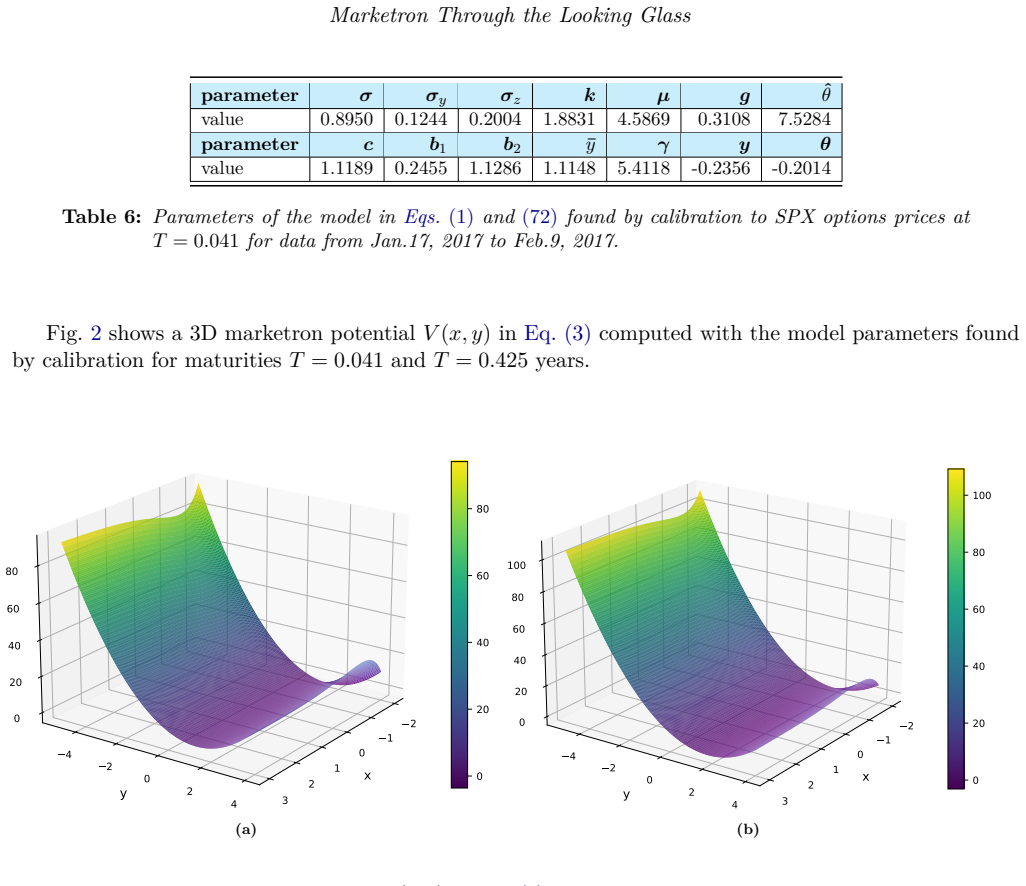
- sigma =
0.3934 (T=0.425), 0.8950 (T=0.041)
- sigma_y =
1.008 (T=0.425), 0.1244 (T=0.041)
- sigma_z =
0.8912 (T=0.425), 0.2004 (T=0.041)
- k =
2.7069 (T=0.425), 1.8831 (T=0.041)
- mu =
4.6154 (T=0.425), 4.5869 (T=0.041)
- g =
0.3173 (T=0.425), 0.3108 (T=0.041)
- theta_hat =
6.9242 (T=0.425), 7.5284 (T=0.041)
- c =
0.8897 (T=0.425), 1.1189 (T=0.041)
- b1 =
0.1220 (T=0.425), 0.2455 (T=0.041)
- b2 =
-0.0549 (T=0.425), 1.1286 (T=0.041)
- y_bar =
1.6208 (T=0.425), 1.1148 (T=0.041)
- gamma =
1.1031 (T=0.425), 5.4118 (T=0.041)
- y(0) =
-0.0589 (T=0.425), -0.2356 (T=0.041)
- theta(0) =
1.1007 (T=0.425), -0.2014 (T=0.041)
assumptions (6)
- domain assumption The Marketron SDEs in Eq. (1) describe the joint dynamics of log-price x, memory y, and signal theta.
- domain assumption The memory variable y and signal theta are non-tradable hidden state variables, making the market incomplete.
- domain assumption Investors have exponential utility with risk aversion gamma.
- ad hoc to paper The f and h functions in Eq. (72) (b1 cos and b2 sin) adequately represent signal effects after simplifying the original 8-parameter specification.
- ad hoc to paper The replacement of V'_M(x) with the R2 regularizer in Eq. (B.2) and of f(theta) with f1(theta) in Eq. (B.10) preserves the pricing content of the original model.
- standard math The dual solution for the optimal investment problem yields the market price of risk, and the resulting indifference price is the correct valuation framework.
invented entities (3)
-
Marketron quasiparticle
-
Memory variable y_t
-
Signal theta_t
Cite this review
Pith. "Pith review of Marketron Through the Looking Glass: From Equity Dynamics to Option Pricing in Incomplete Markets." pith.science (2026). https://pith.science/paper/7POUIQY6
@misc{pith2026250809863,
  author       = {Pith},
  title        = {Pith review of: Marketron Through the Looking Glass: From Equity Dynamics to Option Pricing in Incomplete Markets},
  year         = {2026},
  howpublished = {\url{https://pith.science/paper/7POUIQY6}},
  note         = {Machine review of arXiv:2508.09863}
}
abstract
The Marketron model, introduced by [Halperin, Itkin, 2025], describes price formation in inelastic markets as the nonlinear diffusion of a quasiparticle (the marketron) in a multidimensional space comprising the log-price $x$, a memory variable $y$ encoding past money flows, and unobservable return predictors $z$. While the original work calibrated the model to S\&P 500 time series data, this paper extends the framework to option markets - a fundamentally distinct challenge due to market incompleteness stemming from non-tradable state variables. We develop a utility-based pricing approach that constructs a risk-adjusted measure via the dual solution of an optimal investment problem. The resulting Hamilton-Jacobi-Bellman (HJB) equation, though computationally formidable, is solved using a novel methodology enabling efficient calibration even on standard laptop hardware. Having done that, we look at the additional question to answer: whether the Marketron model, calibrated to market option prices, can simultaneously reproduce the statistical properties of the underlying asset's log-returns. We discuss our results in view of the long-standing challenge in quantitative finance of developing an unified framework capable of jointly capturing equity returns, option smile dynamics, and potentially volatility index behavior.
Figures


Figures from the paper (5 more)


Forward citations
Cited by 1 Pith paper
-
Non-Linear and Meta-Stable Dynamics in Financial Markets: Evidence from High Frequency Crypto Currency Market Makers
High-frequency Uniswap v3 crypto data show non-quadratic potentials, with double-well shapes at short sampling frequencies that the author links to market stress.
Reference graph
Works this paper leans on
-
[1]
Joint calibration to SPX and VIX options with signature-based models
url: https://sites.google.com/site/roughvol/home/risks-1. Cuchiero, C. et al. (2024). “Joint calibration to SPX and VIX options with signature-based models”. In: Mathematical Finance35, 1, pp. 161–213. Cunha Jr, A et al. (2024).CEopt: A MATLAB Package for Non-convex Optimization with the Cross-Entropy Method. ArXiv: 2409.00013.url: https://arxiv.org/abs/2...
arXiv 2024
-
[2]
(A.9) and the integrals of the source term in Appendix A.2
B Calculation of auxiliary integrals This section is dedicated to computing four auxiliary expressionsIf,1,If,2,Iv,1,Iv,2 which we need to evaluate A2 in Eq. (A.9) and the integrals of the source term in Appendix A.2. By definition, they read If,1 = ∫∞ −∞ f(ζ)e −ε(ζ−θl)2− (θ−ζ)2 2σ2 θ∆τ σθ √ 2π∆τ dζ, I v,1 =− ∫∞ −∞ ( 1− g eξ + ¯ϵg )e−ε(ξ−xk)2− (x−ξ)2 2σ2∆...
work page 2025
-
[3]
= 1 2a1(τi) [ 1 + Erf (b1 2θ )] . (B.10) Fig. 8 comparesf(x) andf1(x) forb1 = 0.2. The similar behavior of these functions justifies the substitution of f1(x) for f(x) in our further analysis. f(x) f1(x) -100 -50 0 50 100 0 0.2 0.4 0.6 0.8 1.0 x f Figure 8: Functionsf(x),f 1(x) at b1 = 0.2. Using the same approach as employed for computingI2 in Eq. (B.8),...
work page 1964
Reviewed August 5, 2026 · model on record in the stance chip above.
Discussion (0). Continue with ORCID to comment.