REVIEW 4 major objections 5 minor 75 references
The effect of poloidal magnetic field and helicity injection on a breakout CME
T0 review · 4 major / 5 minor · reviewed 2026-08-15 · deepseek-v4-flash
Pith's one-line read The growth rate of absolute net current helicity, not its magnitude, determines whether a sheared solar arcade erupts as a CME.
desk verdict A solid 2.5D breakout CME parameter study whose ANCH-growth-rate claim overreaches a single-run design; the poloidal-field suppression result is the more defensible new piece. read the letter →
The pith
A machine-rendered reading of the paper's core claim, the machinery that carries it, and where it could break.
The reading
What carries the argument
The load-bearing mechanism is breakout reconnection in a multipolar quadrupole-like arcade: shear flow at the base of the middle arcade builds the azimuthal magnetic field and magnetic pressure; the expanding arcade flattens the overlying X-point, reconnection removes the restraining field, and a flux rope can escape. The diagnostic that carries the argument is the absolute net current helicity, the magnitude of the volume-integrated $\mathbf{B}\cdot\mathbf{J}$ over the arcade region, and in particular its time derivative before the first breakout. The background dipole field is the control parameter that sets the height and connectivity of the arcade, turning a less-than-five-percent field increase into a qualitative change in eruption outcome.
What would settle it
Take one of the three shear speeds, for example 36.2 km/s, and rerun the 2.5D breakout simulation at twice and four times the adaptive-mesh refinement resolution; if the eruption classification flips or the ordering of ANCH slopes (multiple greater than single greater than failed) changes, the central claim that ANCH growth rate controls eruption likelihood is not robust.
Extended reading notes
Core claim
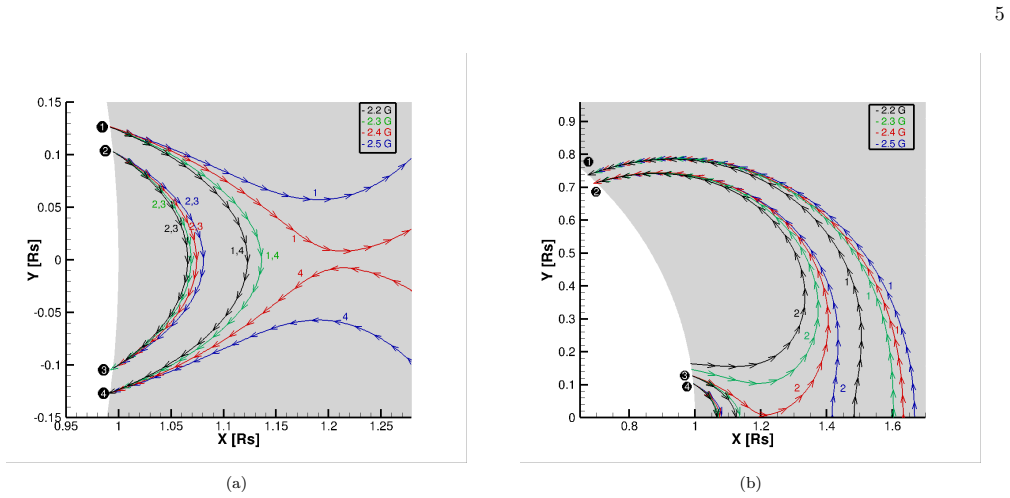
On its own terms, the paper establishes that the breakout CME outcome is set by the balance between helicity injection at the base and the confinement supplied by the background poloidal magnetic field. In simulations with a polar field of 2.2 G, the sheared central arcade forms a flux rope and erupts; at 2.3 G the arcade rises but no flux rope forms; at 2.4–2.5 G even the rise is suppressed, despite a configuration that is otherwise unchanged. With the polar field fixed at 2.2 G, maximum shear speeds of 35.8, 36.2, and 38.8 km s$^{-1}$ yield a failed eruption, a single eruption, and multiple eruptions. Computing the absolute net current helicity $\mathrm{ANCH} = |\sum_i \int \mathbf{B}\cdot\mathbf{J}\,dV|$ across the arcade, the authors find that the slope of ANCH up to the first breakout reconnection orders the three cases: 0.645 (multiple), 0.498 (single), 0.412 (failed) in simulation units. In the multiple-eruption case, the second eruption is preceded by a steeper second rise (0.801), so the rate of increase, not the peak value, is the discriminator. The authors conclude that the ANCH growth rate is the crucial factor determining the likelihood of eruption.
Load-bearing premise
The magnetic reconnection in the simulation is numerical in origin, tied to the grid spacing rather than to a physical resistivity model, so the tiny shear-speed thresholds that define the eruption regimes could shift with resolution.
Editorial extensions
If this is right
- In an active region, a time series of absolute net current helicity should separate eruptive from non-eruptive cases by slope rather than by instantaneous value, giving a possible space-weather precursor.
- Reducing the background poloidal field strength by a few percent makes eruptions easier at the same shear input, consistent with the observed excess of weak CMEs in Solar Cycle 24 under a weakened global magnetic field.
- All breakout CMEs in the investigated domain are slow CMEs, below about 220 km/s, suggesting the mechanism is naturally a source of weak, slow CMEs rather than fast ones.
- The same physical mechanism can produce failed, single, or multiple eruptions under shear-speed differences of only a few km/s, so predicting an eruption requires more than knowing the magnetic configuration at one instant.
Reading between the lines
- Inference: the paper leaves implicit that observational predictors built on SHARP magnetograms should use the time derivative of absolute net current helicity, for example a 6 to 24 hour slope, instead of the snapshot value; this is a direct testable extension.
- Inference: because the regime boundaries sit on shear-speed differences of 0.4 to 2.6 km/s and depend on grid resolution, higher-resolution or three-dimensional simulations will likely shift the exact threshold speeds even if the slope ordering survives.
- Inference: if ANCH growth rate is the controlling factor, then helicity injection history, not just total injected helicity, should enter flare and CME forecasting; an active region that gains helicity quickly should be weighted more heavily than one that gains it slowly.
- Inference: connecting this to Solar Cycle 24, the paper's mechanism suggests the weak-CME excess is physical rather than purely a detection-cadence artifact; a direct observational check would compare ANCH slopes from magnetograms in Cycle 24 and Cycle 23 active regions.
Signed reviews
Editorial analysis
A structured set of objections, weighed in public.
Referee Report
Summary. This manuscript presents 2.5D MHD simulations of breakout CMEs using MPI-AMRVAC. The setup combines a background dipole field with a triple-arcade quadrupolar configuration; after relaxation, a time-dependent shear flow is imposed at the base of the central arcade. Varying the maximum shear velocity (35.8, 36.2, and 38.8 km/s) yields three outcomes: failed eruption, single eruption, and multiple eruptions. The authors also vary the polar background field strength from 2.2 G to 2.5 G and report that stronger poloidal fields suppress eruptions. Tracking global magnetic parameters (excess magnetic energy, total unsigned current helicity, and absolute net current helicity), they conclude that the growth rate of absolute net current helicity (ANCH) is the crucial factor determining eruption likelihood, and they connect this to the excess of weak CMEs in Solar Cycle 24.
Significance. If established, the ANCH-slope criterion would be a practically valuable forecasting precursor, since ANCH-like quantities are available from SHARP photospheric magnetograms. The poloidal-field result is also physically interesting and offers a plausible mechanism for the Solar Cycle 24 weak-CME excess through reduced background field strength. The numerical setup follows established practice (breakout model, AMR, GLM divergence control), and the supplementary movies are a useful resource. However, the central causal claim is not yet supported: the evidence rests on three single runs in which the proposed predictor is controlled by the same input parameter (shear amplitude), and the eruption thresholds are admitted to be resolution dependent. The paper is a worthwhile exploratory study, but the abstract overstates what the simulations demonstrate.
major comments (4)
- [§3.2, Fig. 9, Eq. (8)] The ANCH-slope criterion is collinear with the input shear amplitude. The three scenarios are generated by changing only v0 in Eq. (8) (35.8, 36.2, and 38.8 km/s), and the reported ANCH slopes (0.412, 0.498, and 0.645 in simulation units) increase monotonically with v0. Any monotone diagnostic of injected helicity, such as the slope of magnetic energy or TUCH, would order the three cases in the same way, so the design does not separate the proposed predictor from the control parameter. To support the causal claim, the authors should vary other physical parameters (e.g., background field, heating, or arcade geometry) at fixed v0, or include runs with overlapping ANCH slopes and different outcomes, and compare the discriminative power of ANCH slope against energy slope and TUCH slope in a quantitative analysis.
- [Section 2, final paragraph; §3.2] The eruption thresholds are resolution dependent. The manuscript states that increasing resolution lowers the maximum shearing velocity needed to initiate an eruption, yet the three regime boundaries are separated by only 0.4-2.6 km/s. No convergence study is provided, so the quoted thresholds of 35.8, 36.2, and 38.8 km/s, and hence the associated ANCH slope thresholds, may shift with grid resolution. Without a resolution study, the quantitative slope values in Fig. 9 cannot be distinguished from numerical artifacts. This is a load-bearing issue because the central claim depends on these threshold separations.
- [Section 4, Eqs. (9)-(11)] The forecast link to observations is not established. The simulated ANCH is a coronal volume integral of B·J (Eq. 11), while SHARP ANCH is a photospheric surface quantity. No mapping, unit conversion, or comparison of time evolution between the two is supplied, and the reported slopes are given only in unspecified simulation units. The paper should either provide a forward model connecting the simulated volume quantity to the observable photospheric quantity, or explicitly limit the claim to a qualitative diagnostic hypothesis rather than a ready-to-use forecasting metric.
- [§3.1, Fig. 2] The poloidal-field result is presented mainly through field-line snapshots and qualitative statements. Quantitative eruption metrics for the four Bpol values, such as flux-rope height, velocity, magnetic energy, or helicity budgets, are not reported, and each case is a single run. Since increasing Bpol changes the equilibrium field connectivity (Fig. 1), the claim that a marginal (<5%) change in dipole strength controls eruption likelihood needs quantitative support and a sensitivity check. A quantitative comparison, for example of the maximum central-arcade height or the time of flux-rope formation against Bpol, would make the conclusion much more robust.
minor comments (5)
- [Fig. 6] The text reports velocities for three CMEs in the multiple-eruptions case, but the figure caption and legend appear to show only two curves (first and second CMEs). Please clarify the correspondence and label all curves consistently.
- [Section 2, Eq. (8)] The definition of t0 is confusing: it is first described as the steady-state time (~200 h) and then reset to zero. Please state explicitly that Eq. (8) is evaluated after the reset and remove the ambiguity.
- [Abstract and Section 4] The abstract says the ANCH growth rate 'determines the likelihood' of CME eruptions, while Section 4 says it 'can serve as the most effective indicator.' These are different strengths of claim; please harmonize them and avoid causal wording unless the additional simulations recommended above are performed.
- [Page 1 footnote] The footnote '* Released on March, 1st, 2021' appears to be a leftover from an earlier version and should be removed or updated.
- [Author block] The first author name appears as 'Nitin V ashishtha' with a missing space or title; please check the author block for formatting errors.
Circularity Check
No significant circularity: the ANCH-slope diagnostic is computed from simulated fields, not fitted to, or defined in terms of, the eruption outcome.
full rationale
The paper is a simulation study rather than a fitting exercise. Section 2 prescribes the input shear via Eq. (8) with amplitude v0 and then integrates the MHD equations; the helicity diagnostics Hc, TUCH, and ANCH are defined in Eqs. (9)-(11) as volume integrals over B and J. These are outputs of the simulation, not control parameters, and they are not regressed onto the eruption class. The monotonic ordering of the reported ANCH slopes (0.412, 0.498, 0.645) with v0 (35.8, 36.2, 38.8 km/s) is a physical consequence of increased helicity injection, but no equation in the paper defines the ANCH slope as v0 or as the eruption outcome, so the relationship is not tautological. The conclusion that ANCH growth rate is a useful indicator is an interpretation of the simulated data; its limitations (one varied parameter, three runs, and resolution-dependent thresholds acknowledged in Section 2) concern causal identifiability and numerical robustness, not circularity. The only self-citations, to Talpeanu et al. (2020, 2022), are used for a boundary-condition form and for a similar prior setup, and they are not load-bearing for the central ANCH claim. No circular step can be exhibited from the paper's own equations or reduction chain.
Assumptions & free parameters
free parameters (6)
- Background dipole field strength at poles (Bpol) =
2.2, 2.3, 2.4, 2.5 G (varied across four runs)
- Maximum shear velocity v_phi,max =
35.8, 36.2, 38.8 km/s for failed, single, multiple eruptions
- Arcade vector potential amplitude A0 =
-0.73 G R_sun^5
- Arcade half-width Delta_a =
28.64 deg
- Shear latitude half-width Delta_b =
8.59 deg
- Heating amplitude q0 and target temperatures T0 =
q0=1e6 erg/g/s/K; T0=1.5e6 K (equator), 2.63e6 K (pole)
assumptions (5)
- domain assumption The breakout model of CME initiation (Antiochos et al. 1999) is assumed.
- domain assumption Axisymmetry (2.5D) captures the essential eruption dynamics.
- ad hoc to paper Numerical resistivity provides the reconnection needed for breakout and flare reconnection.
- domain assumption The empirical volumetric heating model produces a realistic bimodal solar wind background.
- domain assumption Global current helicity parameters (TUCH, ANCH) are reliable proxies for CME eruptivity.
Cite this review
Pith. "Pith review of The effect of poloidal magnetic field and helicity injection on a breakout CME." pith.science (2026). https://pith.science/paper/KMPCB3ON
@misc{pith2026250813835,
  author       = {Pith},
  title        = {Pith review of: The effect of poloidal magnetic field and helicity injection on a breakout CME},
  year         = {2026},
  howpublished = {\url{https://pith.science/paper/KMPCB3ON}},
  note         = {Machine review of arXiv:2508.13835}
}
read the original abstract
Coronal mass ejections (CMEs), as crucial drivers of space weather, necessitate a comprehensive understanding of their initiation and evolution in the solar corona, in order to better predict their propagation. Solar Cycle 24 exhibited lower sunspot numbers compared to Solar Cycle 23, along with a decrease in the heliospheric magnetic pressure. Consequently, a higher frequency of weak CMEs was observed during Solar Cycle 24. Forecasting CMEs is vital, and various methods, primarily involving the study of the global magnetic parameters using datasets like Space-weather Helioseismic and Magnetic Imager Active Region Patches (SHARP), have been employed in earlier works. In this study, we perform numerical simulations of CMEs within a magnetohydrodynamics framework using Message Passing Interface - Adaptive Mesh Refinement Versatile Advection Code (MPI-AMRVAC) in 2.5 dimensions. By employing the breakout model for CME initiation, we introduce a multipolar magnetic field configuration within a background bipolar magnetic field, inducing shear to trigger the CME eruption. Our investigation focuses on understanding the impact of the background global magnetic field on CME eruptions. Furthermore, we analyze the evolution of various global magnetic parameters in distinct scenarios (failed eruption, single eruption, multiple eruptions) resulting from varying amounts of helicity injection in the form of shear at the base of the magnetic arcade system. Our findings reveal that an increase in the strength of the background poloidal magnetic field constrains CME eruptions. Furthermore, we establish that the growth rate of absolute net current helicity is the crucial factor that determines the likelihood of CME eruptions.
Figures


Figures from the paper (4 more)


Reference graph
Works this paper leans on
-
[1]
Amari, T., Luciani, J. F., Aly, J. J., Mikic, Z., & Linker, J. 2003a, The Astrophysical Journal, 585, 1073, doi: 10.1086/345501 —. 2003b, The Astrophysical Journal, 595, 1231, doi: 10.1086/377444
-
[2]
Antiochos, S. K. 1998, The Astrophysical Journal, 502, L181, doi: 10.1086/311507
doi:10.1086/311507 1998
-
[3]
Antiochos, S. K., DeVore, C. R., & Klimchuk, J. A. 1999, The Astrophysical Journal, 510, 485, doi: 10.1086/306563
doi:10.1086/306563 1999
-
[4]
Athay, R. G., Gurman, J. B., Shine, R. A., & Henze, W. 1982, ApJ, 261, 684, doi: 10.1086/160379
-
[5]
Athay, R. G., Jones, H. P., & Zirin, H. 1985, ApJ, 288, 363, doi: 10.1086/162799
-
[6]
2012, Solar Physics, 281, 223, doi: 10.1007/s11207-012-9999-3
Poedts, S. 2012, Solar Physics, 281, 223, doi: 10.1007/s11207-012-9999-3
-
[7]
Bobra, M., & Couvidat, S. P. 2014, in AGU Fall Meeting
work page 2014
- [8]
Show all 75 references
-
[9]
G., Sun, X., Hoeksema, J
Bobra, M. G., Sun, X., Hoeksema, J. T., et al. 2014, SoPh, 289, 3549, doi: 10.1007/s11207-014-0529-3
2014 doi
-
[10]
E., Howard, R
Brueckner, G. E., Howard, R. A., Koomen, M. J., et al. 1995, SoPh, 162, 357, doi: 10.1007/BF00733434
1995 doi
-
[11]
1964, in NASA Special Publication, Vol
Carmichael, H. 1964, in NASA Special Publication, Vol. 50, 451
1964
-
[12]
R., & Wilhelm, K
Chae, J., Wang, H., Qiu, J., Goode, P. R., & Wilhelm, K. 2000, ACTIVE REGION LOOPS OBSERVED WITH SUMER ON BOARD THE SOL AR AND HEL IOSPHERIC OBSERV AT ORY Chan´ e, E., Holst, B. V. D., Jacobs, C., Poedts, S., &
2000
-
[13]
2006, Astronomy and Astrophysics, 447, 727, doi: 10.1051/0004-6361:20053802 Chan´ e, E., Poedts, S., & Holst, B
Kimpe, D. 2006, Astronomy and Astrophysics, 447, 727, doi: 10.1051/0004-6361:20053802 Chan´ e, E., Poedts, S., & Holst, B. V. D. 2008, Astronomy and Astrophysics, 492, doi: 10.1051/0004-6361:200811022
2006 doi
-
[14]
1996, Journal of Geophysical Research: Space Physics, 101, 27499, doi: https://doi.org/10.1029/96JA02644
Chen, J. 1996, Journal of Geophysical Research: Space Physics, 101, 27499, doi: https://doi.org/10.1029/96JA02644
1996 doi
-
[15]
Chen, P. F. 2011, Living Reviews in Solar Physics, 8, 1, doi: 10.12942/lrsp-2011-1
2011 doi
-
[16]
2002, Journal of Computational Physics, 175, 645, doi: 10.1006/jcph.2001.6961
Dedner, A., Kemm, F., Kr¨ oner, D., et al. 2002, Journal of Computational Physics, 175, 645, doi: 10.1006/jcph.2001.6961
2002
-
[17]
Domingo, V., Fleck, B., & Poland, A. I. 1995, SoPh, 162, 1, doi: 10.1007/BF00733425
1995 doi
-
[18]
G., & Isenberg, P
Forbes, T. G., & Isenberg, P. A. 1991, ApJ, 373, 294, doi: 10.1086/170051
1991 doi
- [19]
-
[20]
2004, A Global Picture of CMEs in the Inner Heliosphere (Dordrecht: Springer Netherlands), 201–251, doi: 10.1007/978-1-4020-2831-1 8
Gopalswamy, N. 2004, A Global Picture of CMEs in the Inner Heliosphere (Dordrecht: Springer Netherlands), 201–251, doi: 10.1007/978-1-4020-2831-1 8
2004 doi
-
[21]
2010, in Astrophysics and Space Science Proceedings, Vol
Gopalswamy, N., Akiyama, S., Yashiro, S., & M¨ akel¨ a, P. 2010, in Astrophysics and Space Science Proceedings, Vol. 19, Magnetic Coupling between the Interior and Atmosphere of the Sun, 289–307, doi: 10.1007/978-3-642-02859-5 24
2010 doi
-
[22]
2020, in Effect of the Weakened Heliosphere in Solar Cycle 24 on the Properties of Coronal Mass Ejections, Vol
Gopalswamy, N., Akiyama, S., Yashiro, S., et al. 2020, in Effect of the Weakened Heliosphere in Solar Cycle 24 on the Properties of Coronal Mass Ejections, Vol. 1620 (IOP Publishing Ltd), doi: 10.1088/1742-6596/1620/1/012005
2020 doi
-
[23]
2014, Geophysical Research Letters, 41, 2673, doi: 10.1002/2014GL059858
Gopalswamy, N., Akiyama, S., Yashiro, S., et al. 2014, Geophysical Research Letters, 41, 2673, doi: 10.1002/2014GL059858
2014 doi
-
[24]
2006, Space Science Reviews, 123, 303
Gopalswamy, N., Miki´ c, Z., Maia, D., et al. 2006, Space Science Reviews, 123, 303
2006
-
[25]
2015, Astrophysical Journal Letters, 804, doi: 10.1088/2041-8205/804/1/L23
Gopalswamy, N., Xie, H., Akiyama, S., et al. 2015, Astrophysical Journal Letters, 804, doi: 10.1088/2041-8205/804/1/L23
2015 doi
-
[26]
2005, in 29th International Cosmic Ray Conference (ICRC29), Volume 1, Vol
Gopalswamy, N., Xie, H., Yashiro, S., & Usoskin, I. 2005, in 29th International Cosmic Ray Conference (ICRC29), Volume 1, Vol. 1, 169
2005
-
[27]
Gosling, J. T. 1993, Journal of Geophysical Research: Space Physics, 98, 18937, doi: https://doi.org/10.1029/93JA01896 Grigor’ev, V. M., Ermakova, L. V., & Khlystova, A. I. 2007, Astronomy Letters, 33, 766, doi: 10.1134/S1063773707110072
1993 doi
-
[28]
P., Zeeuw, D
Groth, C. P., Zeeuw, D. L. D., Gombosi, T. I., & Powell, K. G. 2000, Journal of Geophysical Research: Space Physics, 105, 25053, doi: 10.1029/2000ja900093
2000 doi
-
[29]
2017, Space Weather, 2399-2891 (IOP Publishing), doi: 10.1088/978-0-7503-1372-8
Hapgood, M. 2017, Space Weather, 2399-2891 (IOP Publishing), doi: 10.1088/978-0-7503-1372-8
2017 doi
-
[30]
Hess, P., & Colaninno, R. C. 2017, ApJ, 836, 134, doi: 10.3847/1538-4357/aa5b85
2017 doi
-
[31]
1974, SoPh, 34, 323, doi: 10.1007/BF00153671
Hirayama, T. 1974, SoPh, 34, 323, doi: 10.1007/BF00153671
1974 doi
-
[32]
2018, Astronomy & Astrophysics, 620, A57, doi: 10.1051/0004-6361/201832976
Hosteaux, S., Chan´ e, E., Decraemer, B., Talpeanu, D.-C., & Poedts, S. 2018, Astronomy & Astrophysics, 620, A57, doi: 10.1051/0004-6361/201832976
2018 doi
-
[33]
2019, Astronomy and Astrophysics, 632, doi: 10.1051/0004-6361/201935894
Hosteaux, S., Chan´ e, E., & Poedts, S. 2019, Astronomy and Astrophysics, 632, doi: 10.1051/0004-6361/201935894
2019 doi
-
[34]
1986, in The Sun and the Heliosphere in Three Dimensions: Proceedings of the XIXth ESLAB Symposium, held in Les Diablerets, Switzerland, 4–6 June 1985, Springer, 107–111 14
Howard, R., Sheeley, N., Michels, D., & Koomen, M. 1986, in The Sun and the Heliosphere in Three Dimensions: Proceedings of the XIXth ESLAB Symposium, held in Les Diablerets, Switzerland, 4–6 June 1985, Springer, 107–111 14
1986
-
[35]
J., Sawyer, C
Hundhausen, A. J., Sawyer, C. B., House, L., Illing, R. M. E., & Wagner, W. J. 1984, Journal of Geophysical Research: Space Physics, 89, 2639, doi: https://doi.org/10.1029/JA089iA05p02639
1984 doi
-
[36]
Jacobs, C., Poedts, S., Holst, B. V. D., & Chan´ e, E. 2005, Astronomy and Astrophysics, 430, 1099, doi: 10.1051/0004-6361:20041676
2005 doi
-
[37]
H., & Sch¨ ussler, M
Jiang, J., Cameron, R. H., & Sch¨ ussler, M. 2015, ApJL, 808, L28, doi: 10.1088/2041-8205/808/1/L28
2015 doi
-
[38]
T., Antiochos, S
Karpen, J. T., Antiochos, S. K., & Devore, C. R. 2012, Astrophysical Journal, 760, doi: 10.1088/0004-637X/760/1/81
2012 doi
- [39]
-
[40]
2000, ApJ, 539, 964, doi: 10.1086/309256
Krall, J., Chen, J., & Santoro, R. 2000, ApJ, 539, 964, doi: 10.1086/309256
2000 doi
-
[41]
2021, The Astrophysical Journal Letters, 917, L29, doi: 10.3847/2041-8213/ac1a15
Li, T., Chen, A., Hou, Y., et al. 2021, The Astrophysical Journal Letters, 917, L29, doi: 10.3847/2041-8213/ac1a15
2021 doi
-
[42]
Lin, J., & Forbes, T. G. 2000, Journal of Geophysical Research: Space Physics, 105, 2375, doi: 10.1029/1999ja900477
2000 doi
-
[43]
2022, Astronomy and Astrophysics, 662, doi: 10.1051/0004-6361/202142868
Liokati, E., Nindos, A., & Liu, Y. 2022, Astronomy and Astrophysics, 662, doi: 10.1051/0004-6361/202142868
2022 doi
-
[44]
T., Valori, G., et al
Liu, Y., Welsch, B. T., Valori, G., et al. 2023, The Astrophysical Journal, 942, 27, doi: 10.3847/1538-4357/aca3a6
2023 doi
-
[45]
G., Petrie, G., & Riley, P
Luhmann, J. G., Petrie, G., & Riley, P. 2013, Journal of Advanced Research, 4, 221, doi: https://doi.org/10.1016/j.jare.2012.08.008
2013 doi
-
[46]
M., Schmieder, B., Ribes, E., & Mein, P
Malherbe, J. M., Schmieder, B., Ribes, E., & Mein, P. 1983, A&A, 119, 197
1983
-
[47]
2007, SOLAR ATMOSPHERIC DYNAMIC COUPLING DUE TO SHEAR MOTIONS DRIVEN BY THE LORENTZ FORCE Manchester IV, W
Manchester, W. 2007, SOLAR ATMOSPHERIC DYNAMIC COUPLING DUE TO SHEAR MOTIONS DRIVEN BY THE LORENTZ FORCE Manchester IV, W. B., Gombosi, T. I., Roussev, I., et al. 2004, Journal of Geophysical Research: Space Physics, 109, doi: https://doi.org/10.1029/2003JA010150
2007 doi
-
[48]
J., Angold, N., Elliott, H
McComas, D. J., Angold, N., Elliott, H. A., et al. 2013, ApJ, 779, 2, doi: 10.1088/0004-637X/779/1/2
2013 doi
-
[49]
2019, ApJ, 880, 51, doi: 10.3847/1538-4357/ab26a7
Michalek, G., Gopalswamy, N., & Yashiro, S. 2019, ApJ, 880, 51, doi: 10.3847/1538-4357/ab26a7
2019 doi
-
[50]
C., & Schnack, D
Mikic, Z., Barnes, D. C., & Schnack, D. D. 1988, ApJ, 328, 830, doi: 10.1086/166341
1988 doi
-
[51]
Mikic, Z., & Linker, J. A. 1994, ApJ, 430, 898, doi: 10.1086/174460
1994 doi
-
[52]
2021, Astronomy and Astrophysics, 649, doi: 10.1051/0004-6361/202140384 Mu˜ noz-Jaramillo, A., Sheeley, N
Moraitis, K., Patsourakos, S., & Nindos, A. 2021, Astronomy and Astrophysics, 649, doi: 10.1051/0004-6361/202140384 Mu˜ noz-Jaramillo, A., Sheeley, N. R., Zhang, J., & DeLuca, E. E. 2012, ApJ, 753, 146, doi: 10.1088/0004-637X/753/2/146
2021 doi
-
[53]
J., & Forsyth, R
Owens, M. J., & Forsyth, R. J. 2013, Living Reviews in Solar Physics, 10, 5, doi: 10.12942/lrsp-2013-5
2013 doi
-
[54]
E., Valori, G., et al
Pariat, E., Leake, J. E., Valori, G., et al. 2017, Astronomy and Astrophysics, 601, doi: 10.1051/0004-6361/201630043
2017 doi
-
[55]
Petrie, G. J. D. 2013, The Astrophysical Journal, 768, 162, doi: 10.1088/0004-637X/768/2/162
2013 doi
-
[56]
Petrie, G. J. D. 2015, ApJ, 812, 74, doi: 10.1088/0004-637X/812/1/74
2015 doi
-
[57]
2023, SoPh, 298, 96, doi: 10.1007/s11207-023-02187-6
Raju, H., & Das, S. 2023, SoPh, 298, 96, doi: 10.1007/s11207-023-02187-6
2023 doi
-
[58]
I., Forbes, T
Roussev, I. I., Forbes, T. G., Gombosi, T. I., et al. 2003, ApJL, 588, L45, doi: 10.1086/375442
2003 doi
-
[59]
I., Sokolov, I
Roussev, I. I., Sokolov, I. V., Forbes, T. G., et al. 2004, ApJL, 605, L73, doi: 10.1086/392504
2004 doi
-
[60]
T., Luhmann, J
Russell, C. T., Luhmann, J. G., & Jian, L. K. 2010, Reviews of Geophysics, 48, RG2004, doi: 10.1029/2009RG000316
2010 doi
-
[61]
Schrijver, C. J. 2015, Socio-Economic Hazards and Impacts of Space Weather: The Important Range between Mild and Extreme, Blackwell Publishing Ltd, doi: 10.1002/2015SW001252
2015 doi
-
[62]
J., & Higgins, P
Schrijver, C. J., & Higgins, P. A. 2015, Solar Physics, 290, 2943, doi: 10.1007/s11207-015-0785-x
2015 doi
-
[63]
2022, The Astrophysical Journal, 935, 45, doi: 10.3847/1538-4357/ac7955
Sinha, S., Gupta, O., Singh, V., et al. 2022, The Astrophysical Journal, 935, 45, doi: 10.3847/1538-4357/ac7955
2022 doi
-
[64]
J., & Balogh, A
Smith, E. J., & Balogh, A. 2008, Geophys. Res. Lett., 35, L22103, doi: 10.1029/2008GL035345 St. Cyr, O., Burkepile, J., Hundhausen, A., & Lecinski, A. 1999, Journal of Geophysical Research: Space Physics, 104, 12493
2008 doi
- [65]
-
[66]
C., Poedts, S., D’Huys, E., & Mierla, M
Talpeanu, D. C., Poedts, S., D’Huys, E., & Mierla, M. 2022, A&A, 658, A56, doi: 10.1051/0004-6361/202141977
2022 doi
-
[67]
2020, A&A, 637, A77, doi: 10.1051/0004-6361/202037477
Talpeanu, D.-C., Chan´ e, E., Poedts, S., et al. 2020, A&A, 637, A77, doi: 10.1051/0004-6361/202037477
2020 doi
-
[68]
2019, Flare-productive active regions, Springer, doi: 10.1007/s41116-019-0019-7 van Ballegooijen, A
Toriumi, S., & Wang, H. 2019, Flare-productive active regions, Springer, doi: 10.1007/s41116-019-0019-7 van Ballegooijen, A. A., & Martens, P. C. H. 1989, ApJ, 343, 971, doi: 10.1086/167766 van der Holst, B., Jacobs, C., & Poedts, S. 2007, The Astrophysical Journal, 671, L77, ...
2019 doi
-
[69]
M., & Colaninno, R
Wang, Y. M., & Colaninno, R. 2014, ApJL, 784, L27, doi: 10.1088/2041-8205/784/2/L27
2014 doi
-
[70]
F., & Howard, T
Webb, D. F., & Howard, T. A. 2012, Living Reviews in Solar Physics, 9, 3, doi: 10.12942/lrsp-2012-3 15
2012 doi
-
[71]
T., Guo, W
Wu, S. T., Guo, W. P., & Dryer, M. 1997, SoPh, 170, 265, doi: 10.1023/A:1004954816406
1997 doi
-
[72]
2004, Journal of Geophysical Research: Space Physics, 109, doi: https://doi.org/10.1029/2003JA010282
Yashiro, S., Gopalswamy, N., Michalek, G., et al. 2004, Journal of Geophysical Research: Space Physics, 109, doi: https://doi.org/10.1029/2003JA010282
2004 doi
-
[73]
2001, Formation of current helicity and emerging magnetic flux in solar active regions
Zhang, H. 2001, Formation of current helicity and emerging magnetic flux in solar active regions. https: //academic.oup.com/mnras/article/326/1/57/1027683
2001
-
[74]
P., Meliani, Z., & Poedts, S
Zuccarello, F. P., Meliani, Z., & Poedts, S. 2012, The Astrophysical Journal, 758, 117, doi: 10.1088/0004-637X/758/2/117
2012 doi
-
[75]
P., Pariat, E., Valori, G., & Linan, L
Zuccarello, F. P., Pariat, E., Valori, G., & Linan, L. 2018, The Astrophysical Journal, 863, 41, doi: 10.3847/1538-4357/aacdfc
2018 doi
Reviewed August 15, 2026 · model on record in the stance chip above.
Discussion (0). Continue with ORCID to comment.