REVIEW 4 major objections 4 minor 34 references
An online-adaptive hyperreduced reduced basis element method for parameterized component-based nonlinear systems using hierarchical error estimation
T0 review · 4 major / 4 minor · reviewed 2026-08-05 · deepseek-v4-flash
Pith's one-line read A component-based reduced-order model can pick, during the solve itself, how fine each part's approximation should be — and thereby meet a 1% error tolerance about 100 times faster than the full simulation.
desk verdict A solid extension of the authors' own HRBE method with a genuinely useful online adaptive fidelity selection, but the error control ultimately rests on an uncertified contraction-factor generalization. read the letter →
The pith
A machine-rendered reading of the paper's core claim, the machinery that carries it, and where it could break.
The reading
What carries the argument
The carrying mechanism is the component-wise hierarchical error estimate of Proposition 1. At each refinement step, the solution at fidelity f is compared with a solution at fidelity f+1; because refinement is assumed to contract the error by an offline-estimated factor η_{bc,f} < 1, the difference between the two solutions, divided by 1 − η, bounds that component's true error, and the sum bounds the system error (Eq. 10). The contraction factors (Eq. 15) are worst-case ratios measured on training subsystems; the hierarchical RB spaces are POD truncations; each fidelity level has its own reduced quadrature rule from component-wise EQP. The Brezzi–Rappaz–Raviart analysis (Corollary 8) keeps h
What would settle it
Assemble a large system (e.g., Nfin=8) with parameters and boundary conditions producing solution features outside the training distribution, run Algorithm 1 to termination, then solve the truth finite-element model and compute the actual error. If any measured per-component contraction ratio ∥u_h − u′_rb∥/∥u_h − u_rb∥ exceeds the offline η_{bc,f}, or if the estimator effectivity (estimate divided by true error) falls below 1 while the algorithm reports convergence, the central assumption is falsified. A cheaper scouting test: record per-component contraction ratios during refinement on a mode
Extended reading notes
Core claim
Component-based reduced models can choose their own component-level fidelity online while still meeting a user-set error tolerance. The engine is a hierarchical estimator (Proposition 1): comparing the current solution (fidelity f) with a one-level-finer solution, scaled by offline-precomputed contraction factors, gives component-wise error bounds whose sum bounds the system error. Refinement starts coarse and enriches only the components with the largest indicators, terminating when the estimate meets tolerance — with no truth solves online. A Brezzi–Rappaz–Raviart analysis couples hyperreduction to RB accuracy so RB fidelity is the single accuracy dial. On thermal-fin systems up to 225 com
Load-bearing premise
The offline-estimated error contraction factors η_{bc,f} — worst-case error-reduction ratios measured over small, randomly assembled training subsystems with random boundary conditions — are assumed to stay valid for the much larger assembled systems and unseen parameters met online; if an online component contracts more slowly than the training worst case, the hierarchical estimator under-predicts the error and the prescribed tolerance can be exceeded.
Editorial extensions
If this is right
- A trained component library can be assembled into new topologies without retraining: the online solve instantiates copies of archetype components and selects their fidelities, so topology changes cost nothing offline.
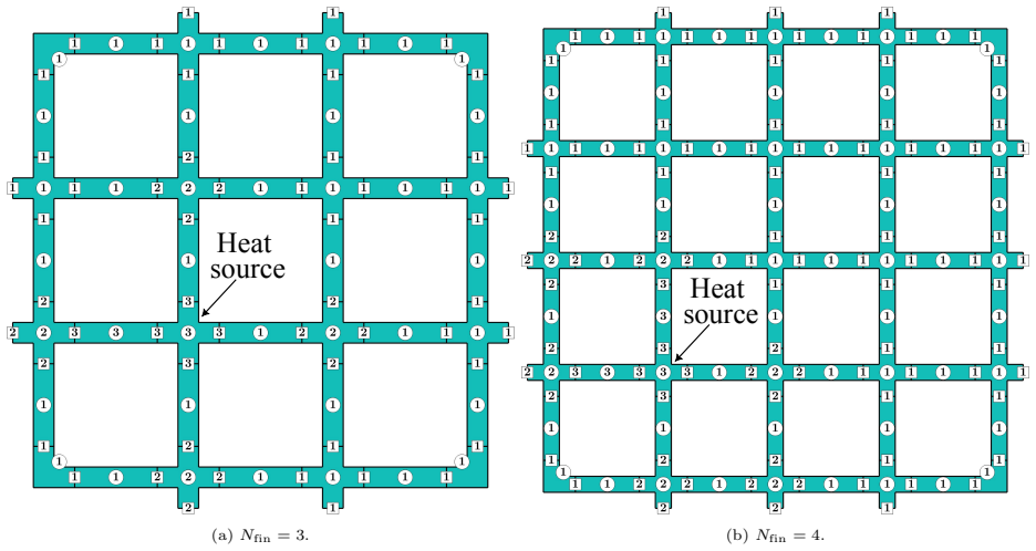
- Large parameter spaces become tractable: the demonstration covers systems with up to 225 components and 68 parameters, with the online problem reduced from roughly 197,000 truth degrees of freedom to about 1,200–1,600.
- Computational savings of O(100) are achievable at 1% error: for the largest tested system the adaptive model reduces degrees of freedom by ≈120–170× and quadrature points by ≈50–70× relative to the truth model.
- Error control is delivered without truth-model access online: the hierarchical estimator's effectivity stays in the range 3–12 across tested systems, and adaptive refinement reaches the 1% target with fewer degrees of freedom than uniform refinement.
- Because hyperreduction accuracy is fixed offline to sit below the RB error, only the RB fidelity needs to be adapted online — the adaptive algorithm has a single accuracy dial to turn.
Reading between the lines
- The paper leaves untested how the contraction factors degrade for assemblies much larger than the training subsystems; a safeguard the analysis suggests is monitoring the observed per-component contraction ratio online and tightening η if it approaches 1.
- For three-dimensional or vector-field problems, the paper notes that building quadrature rules for every multi-indexed fidelity level may become too costly (Remark 9); its fallback of reusing the nearest higher-fidelity RQ rule is not numerically assessed, and the accuracy/cost trade-off of that fallback is a natural next experiment.
- The refinement policy (enrich the top Δ% of components by local indicator) is a heuristic; a cost-weighted selection rule that accounts for the differing cost of refining a cross versus a rod could plausibly beat the reported degree-of-freedom counts at equal accuracy.
- Because the finest library spaces are reserved as the comparison space and never used as the returned solution, the method carries an implicit fidelity ceiling; extending the hierarchy online with freshly generated snapshots is an open direction the paper does not pursue.
Editorial analysis
A structured set of objections, weighed in public.
Referee Report
Summary. The paper develops an online-adaptive hyperreduced reduced basis element (HRBE) method for parameterized, component-based nonlinear systems. Offline, a library of archetype components is equipped with hierarchical RB spaces for bubbles and ports, component-wise empirical quadrature rules, and error contraction factors. Online, an adaptive algorithm (Algorithm 1) starts from coarse component fidelities, solves the HRBE problem at current and refined fidelities, estimates the system-level error using Proposition 1, and selectively refines components until the estimated error falls below a user-prescribed tolerance. The error estimator is a hierarchical estimator based on comparing successive fidelity levels, and the contraction factors used in it are estimated offline from randomly assembled training subsystems. The total error between the HRBE and truth solutions is also analyzed via the Brezzi–Rappaz–Raviart theorem, yielding the bound (14) under residual and nonlinearity assumptions. Numerical experiments on nonlinear thermal fin systems with up to 225 components report O(100) speedup at about 1% error and show that adaptive refinement uses fewer degrees of freedom than uniform refinement.
Significance. If the method performs as claimed, the paper is a useful contribution to component-based model reduction: it extends hyperreduced RB element methods to multi-fidelity online adaptation, introduces a practical hierarchical error indicator, couples hyperreduction accuracy to RB accuracy via the BRR theorem, and demonstrates the methodology on a nontrivial, moderately large nonlinear thermal fin benchmark. The authors are transparent about the offline training assumptions and provide rich numerical evidence, including effectivity plots and component-wise refinement visualizations. The main significance is in the algorithmic framework and its numerical demonstration rather than in a fully certified a posteriori error bound. The paper would be strengthened by clearly separating certified statements from heuristic offline estimates and by validating the load-bearing contraction assumption on held-out configurations.
major comments (4)
- [Section 5.3, Eq. (15); Remark 3] The error-control guarantee of Algorithm 1 rests on Proposition 1, whose first inequality requires the contraction assumption (9) with the offline-estimated factors η_{bc,f}. Equation (15) computes η as the maximum ratio over training subsystems assembled by Algorithm 2, and Section 5.3 explicitly states that it is infeasible to verify the contraction property for all systems and parameters and that generalization is assumed. This is a load-bearing point: if for an online component the actual contraction ratio exceeds η_{M(c),f_c}, the proof of Proposition 1 fails, Eq. (10) under-predicts the error, and Algorithm 1 can stop with true error above the 1% tolerance. The numerical validation uses only five parameter samples per Nfin (Section 7.3.2) and the same offline-estimated η; it does not certify the assumption on unseen topologies/parameters. I recommend either adding a held-out valida
- [Section 6, Eqs. (12)-(14), Propositions 6-7; Remark 3] The BRR-based bound (14) is presented as an a priori error bound, but its ingredients ε_{rb,bc} and eε_{rb,bc} are estimated on training snapshots only, as Remark 3 concedes. Moreover, the nonlinearity conditions (23) and (26) are not verified for any of the numerical experiments. Thus Eq. (14) is not a certified a posteriori bound; it is an offline heuristic used to couple hyperreduction and POD fidelities. This should be stated clearly in the abstract and introduction, where the word 'ensure' appears (e.g., 'to ensure that the user-prescribed system-level error tolerance is met'). The numerical effectivities in Figures 6 and 9 are reassuring, but they do not turn the estimator into a guaranteed bound.
- [Algorithm 1, line 19] Line 19 updates the fidelity using 'fc ← (max(fc,b + 1, Nfdl − 1), ...)'. This should be a minimum, not a maximum. With the max, a selected component already at the highest permissible fidelity Nfdl−1 is moved to Nfdl (the finest level), after which the next iteration's refined space f' = fc+1 is outside the available hierarchy, and Remark 2's restriction is violated. Replacing 'max' with 'min' would correctly cap the fidelity at Nfdl−1. As written, the algorithm can leave itself without a valid refined comparison space.
- [Section 7.3.2, Figures 7-9] The empirical support for the central generalization claim is limited: for each Nfin only five uniformly sampled test parameter tuples are used, and the systems are all of the same regular fin topology. Given that the contraction factors are trained on random small subsystems with random Dirichlet data, the test set does not strongly probe the 'unseen systems and parameters' scenario. Reporting the distribution of actual contraction ratios in (9) or of effectivities over many more random configurations would materially strengthen the claim that the adaptive strategy controls error at the 1% level.
minor comments (4)
- [Section 5.3, Eq. (15)] The denominator in Eq. (15) could be zero if a training HRBE solution exactly matches the truth solution; in practice this does not occur, but a small regularization or a remark would avoid ambiguity.
- [Abstract and Section 4] The phrase 'to ensure that the adaptive strategy meets the desired accuracy' is stronger than what is proved. Suggest replacing 'ensure' with 'estimate' or 'aim to meet' unless a certified bound is added.
- [Section 4.4] The complexity statement 'O(P c N_c,k^2 eQ_c,k) ≪ O(Qh)' mixes asymptotic and non-asymptotic notation. Clarify the constants or state it as an empirical observation.
- [Table 2] The reported range of η (up to 0.998) implies that 1/(1−η) can be as large as 500 for some fidelity transitions. It would be helpful to state whether such transitions are actually encountered during online adaptation or whether the adaptive path avoids them.
Circularity Check
No significant circularity: the hierarchical estimator is a genuine inequality given the contraction factors, and the headline speedup/accuracy claims are checked against the truth FE model.
full rationale
The paper's central derivation, Proposition 1 / Eq. (10), is a valid rearrangement of the assumed contraction inequality (9); it does not reduce by construction to a fitted value. The contraction factors η_{bc,f} are estimated offline via Eq. (15) over training subsystems, and the same η appear in the online estimator and in the validation effectivity plots. This is a training-generalization assumption, not a circular reduction: the estimator is an upper bound, and the reported effectivities 3–12 against truth solutions provide an independent, external check for the tested configurations. The paper explicitly acknowledges the limitation in Remark 3 and Section 5.3, where it states it is 'not feasible to guarantee this contraction behavior for all systems and parameters' and that generalization is assumed. That is a correctness/robustness risk, not a self-definitional or fitted-as-prediction circularity. The method builds on the authors' prior [10] for component-wise EQP and hyperreduction, but [10] is a published, externally available method and is used as a component, not as an unverified self-citation that forces the conclusion. The numerical claims in Section 7 are benchmarked against the truth FE model for fin systems up to Nfin=8 with five random test parameters each, so the O(100) reduction and 1% error results are not manufactured by the estimator. Overall, no step in the derivation chain is equivalent to its own inputs by construction; the score reflects the acknowledged dependence of the error-control guarantee on offline-estimated contraction factors rather than any identified circularity.
Assumptions & free parameters
free parameters (5)
- Error contraction factors eta_{bc,f} =
Max over training set, Eq. (15); reported min 0.207, max 0.998 (Table 2)
- Hyperreduction accuracy ratio e_epsilon/epsilon =
1% (footnote 3 mentions O(10)-O(100))
- POD tolerances delta =
0.1, 0.01, 0.001, 0.0001
- Training-set parameters =
Nsample=100, nu=0.8, random Dirichlet BCs in [1,250] K
- Adaptive refinement parameters =
Nref=10, Delta=10%-20%, tolerance=1%
assumptions (6)
- domain assumption The parametric solution manifold of each archetype component and port is amenable to accurate approximation by low-dimensional linear RB spaces (Section 3.3).
- domain assumption The truth, RB, and HRBE problems are well-posed for all parameters in D (Sections 2.2, 3.2, 3.3).
- domain assumption The training set from Algorithm 2 adequately captures the range of solutions encountered online (Remark 3, Section 5.3).
- domain assumption Error contraction factors estimated on training data generalize to unseen systems and parameters (Section 5.3).
- standard math Brezzi-Rappaz-Raviart regularity conditions (23) and (26) hold, and the truth-to-RB and RB-to-HRBE errors contract as assumed (Propositions 6-7).
- domain assumption Component boundaries are Lipschitz, ports are conformal and mutually separated, and port mappings are geometric-parameter-independent (Section 2.1).
Cite this review
Pith. "Pith review of An online-adaptive hyperreduced reduced basis element method for parameterized component-based nonlinear systems using hierarchical error estimation." pith.science (2026). https://pith.science/paper/75FDC6J5
@misc{pith2026250819027,
  author       = {Pith},
  title        = {Pith review of: An online-adaptive hyperreduced reduced basis element method for parameterized component-based nonlinear systems using hierarchical error estimation},
  year         = {2026},
  howpublished = {\url{https://pith.science/paper/75FDC6J5}},
  note         = {Machine review of arXiv:2508.19027}
}
read the original abstract
We present an online-adaptive hyperreduced reduced basis element method for model order reduction of parameterized, component-based nonlinear systems. The method, in the offline phase, prepares a library of hyperreduced archetype components of various fidelity levels and, in the online phase, assembles the target system using instantiated components whose fidelity is adaptively selected to satisfy a user-prescribed system-level error tolerance. To achieve this, we introduce a hierarchical error estimation framework that compares solutions at successive fidelity levels and drives a local refinement strategy based on component-wise error indicators. We also provide an efficient estimator for the system-level error to ensure that the adaptive strategy meets the desired accuracy. Component-wise hyperreduction is performed using an empirical quadrature procedure, with the training accuracy guided by the Brezzi--Rappaz--Raviart theorem. The proposed method is demonstrated on a family of nonlinear thermal fin systems comprising up to 225 components and 68 parameters. Numerical results show that the hyperreduced basis element model achieves O(100) computational reduction at 1% error level relative to the truth finite-element model. In addition, the adaptive refinement strategy provides more effective error control than uniform refinement by selectively enriching components with higher local errors.
Figures

Figures from the paper (6 more)



Reference graph
Works this paper leans on
-
[1]
M. Barrault, Y. Maday, N. C. Nguyen, and A. T. Patera. An ‘empirical interpolation’ method: appli- cation to efficient reduced-basis discretization of partial differential equations. Comptes Rendus Math- ematique, 339(9):667–672, 2004
work page 2004
- [2]
- [3]
- [4]
-
[5]
A. Buhr. Exponential convergence of online enrichment in localized reduced basis methods. IF AC- PapersOnLine, 51(2):302–306, 2018
work page 2018
-
[6]
G. Caloz and J. Rappaz. Numerical analysis for nonlinear and bifurcation problems. Handbook of Numerical Analysis, 5:487–637, 1997
work page 1997
-
[7]
S. W. Chung, Y. Choi, P. Roy, T. Moore, T. Roy, T. Y. Lin, D. T. Nguyen, C. Hahn, E. B. Duoss, and S. E. Baker. Train small, model big: Scalable physics simulators via reduced order modeling and domain decomposition. Computer Methods in Applied Mechanics and Engineering , 427:117041, 2024
work page 2024
-
[8]
S. W. Chung, Y. Choi, P. Roy, T. Roy, T. Y. Lin, D. T. Nguyen, C. Hahn, E. B. Duoss, and S. E. Baker. Scaled-up prediction of steady Navier-Stokes equation with component reduced order modeling. arXiv preprint arXiv:2410.21534 , 2024
work page Pith review arXiv 2024
Show all 34 references
-
[9]
A. N. Diaz, Y. Choi, and M. Heinkenschloss. A fast and accurate domain decomposition nonlinear manifold reduced order model. Computer Methods in Applied Mechanics and Engineering , 425:116943, 2024
2024
-
[10]
Ebrahimi and M
M. Ebrahimi and M. Yano. A hyperreduced reduced basis element method for reduced-order modeling of component-based nonlinear systems. Computer Methods in Applied Mechanics and Engineering , 431:117254, 2024
2024
-
[11]
J. L. Eftang and A. T. Patera. Port reduction in parametrized component static condensation: approx- imation and a posteriori error estimation. International Journal for Numerical Methods in Engineering , 96(5):269–302, 2013
2013
-
[12]
J. L. Eftang and A. T. Patera. A port-reduced static condensation reduced basis element method for large component-synthesized structures: approximation and a posteriori error estimation. Advanced Modeling and Simulation in Engineering Sciences , 1(1):1–49, 2014
2014
-
[13]
M. A. Grepl, Y. Maday, N. C. Nguyen, and A. T. Patera. Efficient reduced-basis treatment of nonaffine and nonlinear partial differential equations. ESAIM: Mathematical Modelling and Numerical Analysis , 41(3):575–605, 2007
2007
-
[14]
S. Hain, M. Ohlberger, M. Radic, and K. Urban. A hierarchical a posteriori error estimator for the reduced basis method. Advances in Computational Mathematics , 45(5):2191–2214, 2019
2019
-
[15]
J. S. Hesthaven, G. Rozza, and B. Stamm. Certified reduced basis methods for parametrized partial differential equations. Springer, 2016. 31
2016
-
[16]
Hoang, Y
C. Hoang, Y. Choi, and K. Carlberg. Domain-decomposition least-squares Petrov–Galerkin (DD-LSPG) nonlinear model reduction. Computer Methods in Applied Mechanics and Engineering, 384:113997, 2021
2021
-
[17]
D. B. P. Huynh, D. J. Knezevic, and A. T. Patera. A static condensation reduced basis element method: approximation and a posteriori error estimation. ESAIM: Mathematical Modelling and Numerical Anal- ysis, 47(1):213–251, 2013
2013
-
[18]
D. B. P. Huynh, D. J. Knezevic, and A. T. Patera. A static condensation reduced basis element method: Complex problems. Computer Methods in Applied Mechanics and Engineering , 259:197–216, 2013
2013
-
[19]
Iollo, G
A. Iollo, G. Sambataro, and T. Taddei. A one-shot overlapping Schwarz method for component-based model reduction: application to nonlinear elasticity. Computer Methods in Applied Mechanics and Engineering, 404:115786, 2023
2023
-
[20]
M. A. Khamsi and W. A. Kirk. An introduction to metric spaces and fixed point theory . John Wiley & Sons, 2011
2011
-
[21]
A. E. Løvgren, Y. Maday, and E. M. Rønquist. A reduced basis element method for the steady Stokes problem. ESAIM: Mathematical Modelling and Numerical Analysis , 40(3):529–552, 2006
2006
-
[22]
Maday and E
Y. Maday and E. M. Rønquist. A reduced-basis element method. Journal of Scientific Computing , 17(1):447–459, 2002
2002
-
[23]
Maday and E
Y. Maday and E. M. Ronquist. The reduced basis element method: application to a thermal fin problem. SIAM Journal on Scientific Computing , 26(1):240–258, 2004
2004
-
[24]
Aluminum 3003-F (UNS A93003)
National Institute of Standards and Technology. Aluminum 3003-F (UNS A93003). https://www. nist.gov/mml/acmd/aluminum-3003-f-unsa93003 . Accessed: August 2025
2025
-
[25]
Ohlberger and F
M. Ohlberger and F. Schindler. Error control for the localized reduced basis multiscale method with adaptive on-line enrichment. SIAM Journal on Scientific Computing , 37(6):A2865–A2895, 2015
2015
-
[26]
A. T. Patera and M. Yano. An LP empirical quadrature procedure for parametrized functions. Comptes Rendus Mathematique, 355(11):1161–1167, 2017
2017
-
[27]
Quarteroni, A
A. Quarteroni, A. Manzoni, and F. Negri. Reduced basis methods for partial differential equations: an introduction, volume 92. Springer, 2015
2015
-
[28]
Rozza, D
G. Rozza, D. B. P. Huynh, and A. T. Patera. Reduced basis approximation and a posteriori error esti- mation for affinely parametrized elliptic coercive partial differential equations: application to transport and continuum mechanics. Archives of Computational Methods in Engine...
2008
-
[29]
K. Smetana. A new certification framework for the port reduced static condensation reduced basis element method. Computer Methods in Applied Mechanics and Engineering , 283:352–383, 2015
2015
-
[30]
Smetana and A
K. Smetana and A. T. Patera. Optimal local approximation spaces for component-based static conden- sation procedures. SIAM Journal on Scientific Computing , 38(5):A3318–A3356, 2016
2016
-
[31]
Smetana and T
K. Smetana and T. Taddei. Localized model reduction for nonlinear elliptic partial differential equations: localized training, partition of unity, and adaptive enrichment. SIAM Journal on Scientific Computing , 45(3):A1300–A1331, 2023
2023
-
[32]
Veroy and A
K. Veroy and A. T. Patera. Certified real-time solution of the parametrized steady incompressible Navier–Stokes equations: rigorous reduced-basis a posteriori error bounds. International Journal for Numerical Methods in Fluids , 47(8-9):773–788, 2005
2005
-
[33]
E. L. Wilson. The static condensation algorithm. International Journal for Numerical Methods in Engineering, 8(1):198–203, 1974. 32
1974
-
[34]
Yano and A
M. Yano and A. T. Patera. An LP empirical quadrature procedure for reduced basis treatment of parametrized nonlinear PDEs. Computer Methods in Applied Mechanics and Engineering , 344:1104– 1123, 2019. 33
2019
Reviewed August 5, 2026 · model on record in the stance chip above.
Discussion (0). Continue with ORCID to comment.