Pith. sign in

REVIEW 4 major objections 4 minor 14 references

Decompositions of augmentation varieties via weaves and rulings

T0 review · 4 major / 4 minor · reviewed 2026-08-05 · deepseek-v4-flash

Pith's one-line read The paper proves that the ruling, weave, Deodhar, and sheaf decompositions of four isomorphic varieties coincide.

desk verdict A substantial, likely-correct unification of four decompositions of augmentation/braid varieties; the main proof structure holds up, with a few presentation gaps a referee should ask to close. read the letter →

arxiv 2508.20226 v1 pith:S42XUFG4 submitted 2025-08-27 math.SG math.AGmath.COmath.RT

classification math.SGmath.AGmath.COmath.RT
keywords augmentationvarietiesbraidLegendrianlinksnormalrulingsweavesMorsecomplexsequencesDeodhardecompositionmicrolocalsheaves
verification ladder T0 review T1 audit T2 compute T3 formal

The pith

A machine-rendered reading of the paper's core claim, the machinery that carries it, and where it could break.

The reading

The paper proves that four independently defined decompositions of the same algebraic variety agree. Starting from a positive braid β whose Demazure product is the longest permutation, one can form the augmentation variety of the Legendrian (−1)-closure of βΔ, the braid variety of β, an open Richardson-type braid-Richardson variety, and a framed moduli space of microlocal rank-1 sheaves; each carries a decomposition into pieces of the form (C*)^t × C^c. The decompositions come from normal rulings, simplifying weaves, distinguished sequences of permutations, and ruling-type data on sheaves. The paper shows all four decompositions coincide under the known isomorphisms, so point counts, dimensions, and Hodge-theoretic information extracted from any one of them are the same. The proof works by comparing weaves with Morse complex sequences through a braid category whose morphisms are sequences of braid moves.

What carries the argument

The carrying mechanism is a pair of categories connected by a functor A: the braid category B_n of sequences of positive braids related by braid moves, and the weave category W_n of algebraic weaves. Another functor M sends each morphism to an algebraic correspondence built from Morse complex sequences with trivial monodromy; Theorem 4.31 proves M = X ∘ A. This identifies the trivial-monodromy equations of weaves with explicit handleslide relations in Morse complex sequences, putting the ruling decomposition and the weave decomposition on the same footing. The load-bearing bijection is Lemma 4.45, between normal rulings of Λ(βΔ) and inductive equivalence classes of right simplifying weaves β

What would settle it

Compute, for a positive braid β with δ(β)=w0 that is not of the form Δγ, the number and dimensions of the pieces in the ruling decomposition of Aug(Λ(βΔ)) and in the weave decomposition of X(β) by right simplifying weaves; the theorem predicts matching counts with switches corresponding to trivalent vertices and returns (minus the crossings of Δ) corresponding to cups, so any disagreement in the strata or in their point counts over finite fields would falsify it.

Watch

Extended reading notes

Core claim

For every positive braid β with Demazure product w0, the ruling decomposition of Aug(Λ(βΔ)) coincides, under the isomorphism α, with the weave decomposition of X(β) by right simplifying weaves (Theorems 1.2 and 4.61); the same pieces are also the Deodhar decomposition of R°_{w0,β} and the sheaf decomposition of M^fr_1(Λ(βΔ)) (Theorem 1.1). The engine is a bijection matching each normal ruling ρ to an inductive equivalence class of right simplifying weaves: switches become trivalent vertices, departures cups, remaining crossings returns. Proof: verify normality in three local cases, then use trivial-monodromy Morse complex sequences to show the two injections have the same image. A byproduct

Load-bearing premise

The whole comparison depends on a combinatorial dictionary that pairs every normal ruling of the Legendrian front with a class of simplifying weaves; if that dictionary ever failed, the four decompositions could describe the same underlying variety but be indexed by different pieces.

Editorial extensions

If this is right

  • Point counts over finite fields, mixed Hodge structures, and homological information extracted from the augmentation variety, braid variety, braid-Richardson variety, or sheaf moduli space are identical, so a computation can be done in whichever language is easiest.
  • Normal rulings of Λ(βΔ) enumerate the pieces of the Deodhar decomposition of R°_{w0,β}, giving a purely Legendrian description of those Deodhar pieces.
  • Cluster variables of the maximal cluster torus of the braid variety can be computed by an explicit algorithm from the formal framed SR-form Morse complex sequence of the maximally switched ruling, so cluster coordinates carry contact-geometric meaning.
  • The 'representations are sheaves' correspondence for these Legendrian weaves is realized by a direct combinatorial comparison, and it is compatible with both the sheaf and ruling decompositions of the augmentation variety.
  • For braids not of the form β = Δγ, the isomorphism between braid variety and augmentation variety now carries a matching stratification, extending results previously known only in the rainbow-closure case.

Reading between the lines

Editorial extensions of the paper, not claims the author makes directly.

  • If the bijection between rulings and right simplifying weaves is canonical up to weave equivalence, as the paper expects in Remark 1.6, the common decomposition becomes a Legendrian-isotopy invariant that could distinguish Legendrian links with the same classical invariants.
  • The Morse-complex algorithm for cluster variables likely extends beyond the maximal cluster torus, since the handleslide relations under MCS braid moves transform variables by Laurent monomials of the same shape as cluster mutations.
  • The agreement of the sheaf and ruling decompositions suggests that microlocal sheaf computations for these Legendrians could be replaced by the finite combinatorics of normal rulings, making sheaf-theoretic invariants accessible for larger braids without building sheaves by hand.
Share X Bluesky LinkedIn Reddit HN

Editorial analysis

A structured set of objections, weighed in public.

Desk editor's note, referee report, and a circularity audit.

Referee Report

4 major / 4 minor

Summary. The paper proves that several decompositions of the augmentation variety of a Legendrian (−1)-closure Λ(β∆) coincide under known isomorphisms with the braid variety X(β), the braid-Richardson variety R°_{w0,β}, and the framed moduli space of microlocal rank-1 sheaves. The main theorem (Theorem 1.1, with detailed versions Theorems 1.2–1.5) asserts that the ruling decomposition, the weave decomposition, the Deodhar decomposition, and the sheaf decomposition are all the same decomposition. The proof introduces a braid category B_n with moves corresponding to algebraic weaves, constructs a functor A : B_n → W_n and a functor M : B_n → C via Morse complex sequences, and proves that the trivial-monodromy varieties agree (Theorem 4.31). The key index-matching step is a claimed bijection between normal rulings of Λ(β∆) and inductive equivalence classes of right simplifying weaves β → ∆ (Lemma 4.45). The paper also gives an MCS-combinatorial algorithm for cluster variables of the maximal cluster torus and discusses cycle deletion.

Significance. If the main theorem is correct, it unifies four a priori different algebraic decompositions of the same underlying variety, and it gives a new combinatorial way to compute cluster variables from rulings via Morse complex sequences. The categorical framework—the braid category, the functors A and M, and the comparison M(m) ≅ X(A(m))—is a reusable contribution, and the paper contains several explicit computations (e.g., Examples 4.59, 4.65, 4.82) that illustrate the constructions well. The result is likely to be of interest to symplectic geometers and cluster algebraists. However, the central combinatorial bijection in Lemma 4.45 is not fully proved, and some of the sheaf-theoretic decomposition statements are imported with only sketches; these issues affect load-bearing steps of Theorems 4.61 and 4.89.

major comments (4)
  1. [§4.3, Lemma 4.45]
  2. [§4.3, Proposition 4.43]
  3. [§3.5, Theorem 3.57]
  4. [§4.5, Theorem 4.88]
minor comments (4)
  1. [§2.5, Notation 2.24] The definition of ∂D^2_- repeats '{z > 0}'; it should presumably be '{z < 0}'.
  2. [Examples 3.27 and 4.80] There is a sign inconsistency in the computation of A_2: Example 3.27 gives A_2 = z_2 z_3 − 1, while Example 4.80 gives A_2 = 1 − z_2 z_3, and the alternative computation in Example 4.65 also concludes 1 − z_2 z_3 although the displayed formula gives z_2 z_3 − 1. These should be reconciled.
  3. [§2.7, Theorem 2.39 proof] The sentence 'it suffices to prove that there is an somorphism Aug(Λ(β∆)) ∼= Aug(Λpig(Λ(β∆))' contains a typo: 'somorphism' and an extra 'Λ' in the second argument.
  4. [§3.6, Theorem 3.67] The proof of Theorem 3.67 is omitted with the explanation that it follows from Theorem 3.69, while Theorem 3.69 is later proved by induction using Lemma 3.66. This organization is acceptable, but the cross-reference should be clarified to avoid the appearance of circularity.

Circularity Check

0 steps flagged · score 2.0 of 10

No significant circularity: the central decomposition comparison is proved by matching pieces via new bijections; self-citations are minor and not load-bearing.

full rationale

The central claim, that the ruling, weave, Deodhar, and sheaf decompositions coincide, is not assumed as an input. The paper imports the four decompositions from external or prior work ([HR15b], [CGGS24], [GLTW24]/[Deo85], [STZ17]) and then proves the coincidence by constructing explicit bijections between index sets and commutative diagrams of injective maps. In particular, Theorem 4.61 relies on Lemma 4.45, which proves a bijection between normal rulings and inductive equivalence classes of right simplifying weaves by assigning local labels (switch/departure/return) from the weave data and checking local normality via the Demazure product; this is a novel combinatorial argument rather than a restatement of the theorem. The equality of piece images is then established by Theorem 4.60's commutative diagram using the explicitly defined maps ψ_r and η_ρ, not by definition of the decompositions. The paper does contain self-citations: Proposition 2.42 says the sheaf-space isomorphism is 'essentially contained in [CL22, Corollaries 6.3 and 6.6] or [CW24, Lemma 4.3 and Proposition 4.4], but we provide a direct proof here for exposition.' This is a self-citation, but the proposition is reproved and the cited facts are standard flag/sheaf identifications, not the final decomposition comparison, so it is not load-bearing. The only self-referential note is before Theorem 3.67: 'We omit the proof of the following theorem since it follows from the identification with the weave decomposition in Theorem 3.69.' This could look like a circular dependency, but Theorem 3.67 is an external Deodhar decomposition result, and Theorem 3.69's proof independently matches the Deodhar pieces to weave pieces by induction using Lemma 3.66. Thus the omitted proof does not reduce the paper's conclusions to its own assumptions. A correctness skeptic could question whether Lemma 4.45's local normality checks assemble into a global ruling, but that is a gap in proof detail, not circularity: no equation is defined in terms of the target result, and no fitted parameter is renamed as a prediction. Overall, the derivation chain is self-contained against external benchmarks for the main comparison.

Assumptions & free parameters 0 free parameters · 4 assumptions · 0 invented entities

No new physical entities or ad hoc parameters. The free variables in braid matrices and MCS handleslide marks are coordinates on the varieties, not fitted constants. The paper's new objects (braid category Bn, functors A and M) are mathematical constructions, not invented entities.

assumptions (4)
  • domain assumption Henry-Rutherford's ruling decomposition and MCS/A-form isomorphisms hold over C with the sign conventions used here.
    Invoked in Theorems 3.40, 3.44, 3.47, and 3.56; the paper modifies signs (Remarks 3.29, 3.37) and claims the proofs go through over any commutative ring (Remark 3.43).
  • domain assumption Casals-Gorsky-Gorsky-Simental's weave decomposition and the functor X: Wn → C exist and are injective on pieces.
    The weave decomposition (Theorem 3.13) and algebraic weave correspondences (Theorem 3.12) are imported from [CGGS24].
  • domain assumption Shende-Treumann-Zaslow's ruling decomposition of the moduli space of microlocal rank-1 sheaves extends from rainbow closures to (−1)-closures of β∆.
    Theorem 3.57 restates this generalization with a proof sketch; it is needed for Theorem 1.5 and Theorem 4.89.
  • domain assumption Equivalence of augmentations and microlocal sheaves for the considered Legendrians (NRS+20, RS18, RS19, and related works).
    Used in Section 4.5, especially Theorem 4.87, to map between MC2Fs and simple sheaves.

how reviews work

0 comments
Cite this review

Pith. "Pith review of Decompositions of augmentation varieties via weaves and rulings." pith.science (2026). https://pith.science/paper/S42XUFG4

@misc{pith2026250820226,
  author       = {Pith},
  title        = {Pith review of: Decompositions of augmentation varieties via weaves and rulings},
  year         = {2026},
  howpublished = {\url{https://pith.science/paper/S42XUFG4}},
  note         = {Machine review of arXiv:2508.20226}
}
read the original abstract

The braid variety of a positive braid and the augmentation variety of a Legendrian link both admit decompositions coming from weaves and rulings, respectively. We prove that these decompositions agree under an isomorphism between the braid variety and the augmentation variety. We also prove that both decompositions coincide with a Deodhar decomposition and another decomposition coming from the microlocal theory of sheaves. Our proof relies on a detailed comparison between weaves and Morse complex sequences. Among other things, we show that the cluster variables of the maximal cluster torus of the augmentation variety can be computed from the Legendrian via Morse complex sequences.

Figures

Figures reproduced from arXiv: 2508.20226 by the authors.

Figure 1
Figure 1. The correspondence between trivial monodromy weaves and Morse complex sequences. The dashed handleslide marks and marked points (on the right) are related to the horizontal dashed segments in the weave (on the left). Remark 1.6. The collection of right simplifying weaves that we construct is not unique. However, any such collection corresponding to the normal rulings obtained by the map ρ 7→ wρ induces the same weav… view at source ↗
Figure 2
Figure 2. Left: A normal ruling ρ of the Legendrian (−1)-closure of (σ 2 1σ 2 2 ) 2∆. Right: The corresponding right simplifying weave wρ. The la￾bels “s” and “d” denote switches and departures, respectively. Associated to the normal ruling ρ of Λ(β∆), Henry–Rutherford [HR15b] defined an injective map ϕρ : C r(ρ)−( n 2 ) × (C ∗ ) s(ρ) ,−→ Aug(Λ(β∆)), and we compare this injective map with the injective map ϕrρ induced by M(rρ… view at source ↗
Figure 3
Figure 3. The front projection of the (−1)-closure of β (in plat position). Definition 2.4 (Nearly plat). Let D be the front diagram of a Legendrian link Λ ⊂ R 3 . We say the front diagram D is in nearly plat position if every cusp (both left and right cusps) and every crossing has a distinct x-coordinate. 2.3. Normal rulings. In this section we briefly review the definition of a (graded) normal ruling, independently introduc… view at source ↗
Figures from the paper (52 more)
Figure 4
Figure 4. Figure 4: All the possible configurations of a normal ruling near a crossing. The top row gives all possible configurations near switches, the second row configurations near departures, and the third row near returns. Notation 2.9. Let D be the front diagram of a Legendrian link…
Figure 5
Figure 5. Figure 5: Before and after a number of Reidemeister 2-moves. disks intersect (counted left to right), cp is forced to be a return. Otherwise, we define cp to be a switch. This is uniquely maximal. □ 2.4. Augmentation varieties. One method of finding invariants of Legendrian link…
Figure 6
Figure 6. Figure 6: Transformation of the front of Λ(β∆) under the contactomorphism ϕ to the front diagram ( ∆ β ) Λ . Lemma 2.20. Let β ∈ Br+ n . There is an isomorphism (2.3) V(Λ(β∆)) ∼= Aug(β∆) × C( n 2 ) . Proof. First, we consider a Legendrian isotopy obtained by moving the teardrops…
Figure 7
Figure 7. Figure 7: A Legendrian isotopy followed by the contactomorphism ϕ relating Λ(β∆) and ΛLag( ∆β). ±1 correspond to crossings that are not in the braid word β∆. Under this transformation, they map to the degree ±1 generators of A(ΛLag( ∆))β . In the case where β = ∆γ, it is simple …
Figure 8
Figure 8. Figure 8: The two types of vertices in a weave. weave” and the corresponding graph is an “n-graph.” We have instead chosen to adopt the terminology of [CGGS24, CGGS21, CGG+25b] and refer to the graph itself as a weave in order to better reflect our focus on braid varieties and t…
Figure 9
Figure 9. Figure 9: Horizontal composition of weaves. Following [CGGS24, Section 4], we now define sliced weaves, Demazure weaves, and sim￾plifying weaves. Definition 2.25 (Sliced weave [CGGS24, Definition 4.2]). For a positive braid β ∈ Br+ n , a sliced weave w is a weave β → β ′ that is…
Figure 10
Figure 10. Figure 10: Vertical composition of weaves. • merges three adjacent strands into a hexagonal vertex; Figure 11C for the example with strands GiGi+1Gi. The case for Gi+1GiGi+1 is analogous. • merges two adjacent strands into a cup; Figure 11D. • merges two adjacent strands into a …
Figure 11
Figure 11. Figure 11: Local models for sliced weaves. Definition 2.26 (Demazure and simplifying weaves). Let β ∈ Br+ n . (1) A simplifying weave is a sliced weave β → δ(β) without any caps. (2) A Demazure weave is a simplifying weave β → δ(β) without any cups. Definition 2.27. We say that …
Figure 12
Figure 12. Figure 12: Defining local models for a right simplifying weave. We now introduce an equivalence relation on the set of right simplifying weaves. By con￾struction any right simplifying weave w is given by wr ◦ · · · ◦ w1, where each wi contains exactly one of the local models dep…
Figure 13
Figure 13. Figure 13: The Lagrangian projection of the Legendrian pigtail closure Λpig(β∆). Proposition 2.37. Let β ∈ Br+ n be such that δ(β) = w0. There is an isomorphism X(β) ∼= Aug(Λpig(β∆)) such that the braid matrix variables are mapped to the corresponding degree 0 generators of A(Λp…
Figure 14
Figure 14. Figure 14: Dashed rays at a trivalent vertex, cup, and cap, respectively. See Figures 1 and 16 for two examples of algebraic weaves. The algebraic weave in [PITH_FULL_IMAGE:figures/full_fig_p025_14.png]
Figure 15
Figure 15. Figure 15: Variables associated to weave segments near a trivalent vertex, hexavalent vertex, and a cup, respectively. Definition 3.11 (Weave category). Let n ∈ Z≥1. Let Wn be the category defined as follows: Objects: Ob(Wn) = Br+ n . Morphisms: A morphism β1 → β2 is an algebrai…
Figure 16
Figure 16. Figure 16: A framed right inductive weave with trivial monodromy. The highlighted edge is the only Lusztig cycle that covers. 3.3. Morse complex sequences. Morse complex sequences, which were first introduced in unpublished work of Pushkar′ , and in print by Henry [Hen11, Sectio…
Figure 17
Figure 17. Figure 17: The different kinds of tangles Dℓ used to define dℓ and φℓ . Definition 3.31 (Simple left cusp). Let C be an MCS over R for a front diagram D equipped with a Maslov potential. A simple left cusp for C is a left cusp in D (see Figure 17C) such that ⟨dℓ+1e(ℓ + 1)j , e(ℓ…
Figure 18
Figure 18. Figure 18: MCS moves. Near switches: One handleslide mark immediately to the left and one handleslide mark immediately to the right of every switch equipped with the elements r ∈ R∗ and −r −1 ∈ R∗ , respectively. Moreover, there is one more handleslide mark between the two “comp…
Figure 19
Figure 19. Figure 19: MCS moves involving marked points. are nested or disjoint (see the third row of [PITH_FULL_IMAGE:figures/full_fig_p035_19.png]
Figure 20
Figure 20. Figure 20: Local models for the SR-form MCS associated to a normal rul￾ing. The thickness of the lines indicate the boundaries of the two ruling disks. A dotted arrow between strands j and k for j < k with label x means ⟨dℓe(ℓ)k, e(ℓ)j ⟩ = x. Remark 3.36. A handleslide mark equi…
Figure 21
Figure 21. Figure 21: Braid moves algebraic weaves with no caps). Then it is clear that A restricts to an equivalence of categories A: B∪ n ∼=−→ w∪ n . 4.2. Monodromy of Morse complex sequences. The next goal is to define a functor Bn → C, where C is the category of algebraic correspondenc…
Figure 22
Figure 22. Figure 22: MCS Braid moves Remark 4.7. We colloquially call the handleslide marks indicated with dashed lines on the right side of Figures 22C and 22D “dashed handleslide marks” and call the labeled dots “marked points.” Given a Morse complex sequence C as in Definition 3.28, wh…
Figure 23
Figure 23. Figure 23: MCS moves with trivial monodromy. Let m: β → β ′ be a morphism in the braid category, i.e., a sequence of braids (β1, . . . , βq) from β to β ′ and a sequence of braid moves. Let p ∈ {2, . . . , q}. If βp is obtained from βp−1 by a trivalent move or a cup move, then β…
Figure 24
Figure 24. Figure 24: The associated A-form MCS sequence with trivial monodromy for the morphism σ1σ2σ 2 1σ2 → ∆ with braid sequence (β1 = σ1σ2σ 2 1σ2, β2 . . . , β5 = ∆). Here V is the monodromy associated with all the residual dashed handleslide marks and marked points that are located t…
Figure 25
Figure 25. Figure 25: Choosing y ∈ C ∗ arbitrarily determines the handleslide marks before the MCS trivalent move. after the backwards MCS trivalent move are determined by the condition that the monodromy is the identity; see Lemma 4.19. Similarly, for the MCS cup move, we choose x ∈ C arb…
Figure 26
Figure 26. Figure 26: Choosing x ∈ C arbitrarily determines the handleslide marks before the MCS cup move. (3) For m: β → ∆, since X(∆) may be identified with the origin in C( n 2 ) , the map ϕm is defined as the composition C c × (C ∗ ) t −→ C c × (C ∗ ) t × {0} −→ X(β) and is injective b…
Figure 27
Figure 27. Figure 27: Top: A framed A-form MCS. Bottom: An unframed A-form MCS. All variables at handleslide marks and marked points are omitted. (3) A framed MCS trivalent move is the local modification of the front diagram of a framed MCS defined by Figure 28C. (4) A framed MCS cup move …
Figure 28
Figure 28. Figure 28: Framed MCS braid moves. (2) The monodromy of each framed MCS move required to move the dashed handleslide marks to the right of the rightmost crossing of βj , is equal to the identity matrix. (3) The matrix µ(β ′ )π is upper triangular. We use the notation Mfr(m) := M…
Figure 29
Figure 29. Figure 29: Framed MCS braid moves with trivial monodromy. Theorem 4.40. Let n ∈ Z≥1. For any β ∈ Br+ n , there is a functor Mfr : Bn → C such that Mfr(β) = M(β) = X(β) and a functor Xfr : Wn → C such that Xfr(β) = X(β) = X(β). In [PITH_FULL_IMAGE:figures/full_fig_p058_29.png]
Figure 30
Figure 30. Figure 30: A normal ruling ρ of the (−1)-closure of (σ 2 1σ 2 2 ) 2∆. The crossings marked with points represent the switches [PITH_FULL_IMAGE:figures/full_fig_p062_30.png]
Figure 31
Figure 31. Figure 31: A right inductive morphism rρ : β → ∆ in the ruling category associated to the normal ruling ρ of Λ(β∆) shown on the top braid by the crossings with marked points representing the switches. In each step, the gray rectangle indicates which MCS braid move is performed. …
Figure 32
Figure 32. Figure 32: The weave A(rρ) is a right simplifying weave on β. t2 t1 x y −→ a −a b −1 t2 t1 [PITH_FULL_IMAGE:figures/full_fig_p063_32.png]
Figure 33
Figure 33. Figure 33: The MCS-SR trivalent move. SR(r) := (SR(β1), . . . , SR(βq)) of formal SR-form MCSs such that for each j ∈ {2, . . . , q} exactly one of the following holds: (1) SR(βj−1) is related to SR(βj ) via an MCS distant crossings move or a MCS hexavalent move. (2) SR(βj−1) is…
Figure 34
Figure 34. Figure 34: MCS-SR trivalent move with trivial monodromy. Notation 4.52. Let r: β → ∆ be a morphism in Rn with c cups, t trivalent moves and underlying ruling ρ. Recall the notation used in (4.1). We define Mρ (r) ⊂ V r := C L ×  C( n 2 ) × (C ∗ ) n R to be the algebraic subvar…
Figure 35
Figure 35. Figure 35: A backwards MCS-SR trivalent move with trivial monodromy used to define the map ψr . Lemma 4.53. Let r: β → ∆ be a morphism in Rn with c cup moves, t trivalent moves and underlying normal ruling ρ. There is an injective composition ψr : C c × (C ∗ ) t ∼=←− Mρ (r) −→ M…
Figure 36
Figure 36. Figure 36: The morphism rρ [PITH_FULL_IMAGE:figures/full_fig_p065_36.png]
Figure 37
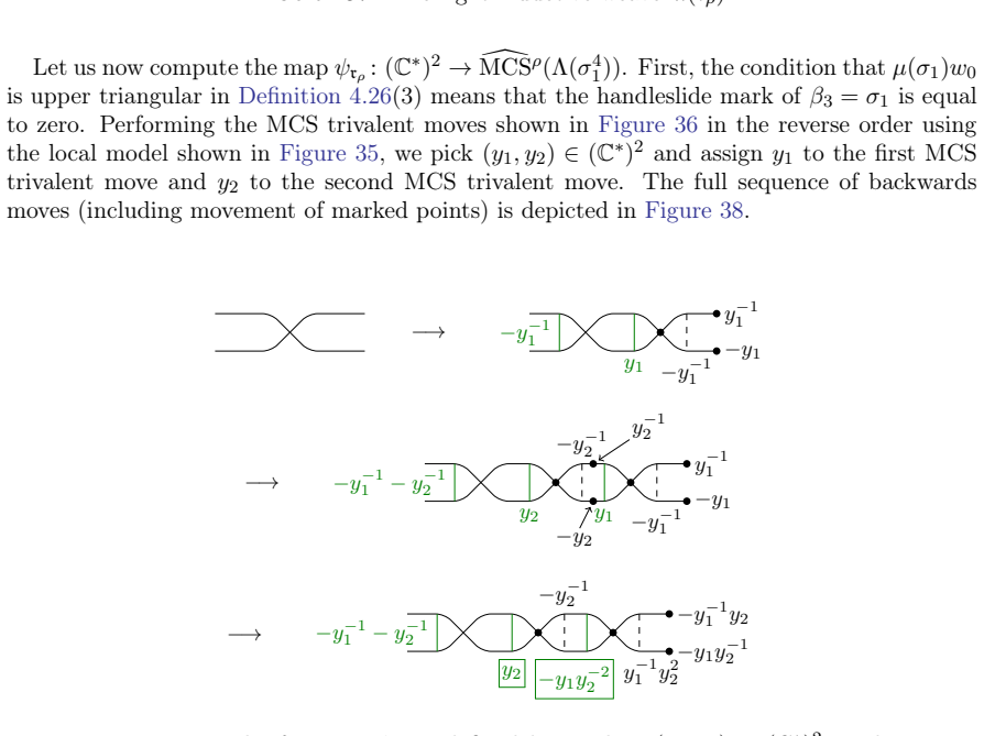
Figure 37. Figure 37: The right inductive weave A(rρ). Let us now compute the map ψrρ : (C ∗ ) 2 → MCS [ρ (Λ(σ 4 1 )). First, the condition that µ(σ1)w0 is upper triangular in Definition 4.26(3) means that the handleslide mark of β3 = σ1 is equal to zero. Performing the MCS trivalent moves…
Figure 38
Figure 38. Figure 38: The function ψrρ is defined by sending (y1, y2) ∈ (C ∗ ) 2 to the equivalence class of the SR-form MCS associated to the normal ruling ρ de￾picted at the bottom. The map η −1 ρ : MCS [ρ (Λ(σ 4 1 )) → (C ∗ ) 2 is given by picking out the handleslide mark at each return…
Figure 39
Figure 39. Figure 39: The inverse to ψrρ is defined by sending an equivalence class of a SR-form MCS to (−y 2 z, y) ∈ (C ∗ ) 2 . trivalent move in the reverse order as indicated by [PITH_FULL_IMAGE:figures/full_fig_p067_39.png]
Figure 40
Figure 40. Figure 40: The sequence of framed A-form MCSs induced by m in Exam￾ple 4.65. The labels which are used to find the s-variables associated to the framed MCS trivalent moves are indicated in boxes. We now show that the s-variables are related to the A-to-SR-form algorithm used in …
Figure 41
Figure 41. Figure 41: The formal framed A-form MCS of the (−1)-closure of σ1σ2σ 3 1σ1(σ2σ 2 1 ) 2 . Recall from Proposition 2.11 that for any β ∈ Br+ n with δ(β) = w0, the (−1)-closure of β∆ admits a unique normal ruling with the maximal number of switches. Definition 4.68 (Formal framed S…
Figure 42
Figure 42. Figure 42: Creation of canceling handleslide marks in the A-to-SR-form al￾gorithm According to the proof of Proposition 4.43, a right inductive morphism rρ performs (framed) MCS trivalent moves with trivial monodromy at the leftmost switch and proceeds right to left [PITH_FULL_…
Figure 43
Figure 43. Figure 43: B, respectively. The crossings marked with • are the switches of the maximally z1 − z2 − z3 − z4 − z5 − z6 − z7 − z8 − (A) z1 − z2 − z3 − z4 − w − z6 − v − z8 − v −1 − w = z5 + z −1 2 (1 − z3z4) v = z7 − z −1 2 z3z6 + z −1 4 (1 − z6w) (B) [PITH_FULL_IMAGE:figures/ful…
Figure 44
Figure 44. Figure 44: The Lusztig cycles in a right inductive morphism of the maxi￾mally switched normal ruling of Λ((σ 2 1σ 2 2 ) 2∆) for the three trivalents which cover another trivalent. Each Lusztig cycle corresponds to one of the colors of sequences of encircled crossings [PITH_FULL…
Figure 45
Figure 45. Figure 45: The MC2F associated to the MCS hexavalent move with trivial monodromy, where the thick green lines depict the handleslide sets in [RS18, Definition 4.1] and the green dot depicts the pentavalent vertex in the han￾dleslide set of the MC2F [RS18, Axiom 4.2(1)]. Corollar…
Figure 46
Figure 46. Figure 46: The MC2F associated to the MCS trivalent move with trivial monodromy, where the thick green lines depict the handleslide sets in [RS18, Definition 4.1], the three green dots depict the pentavalent vertices in the handleslide set [RS18, Axiom 4.2(1)], the cusp points o…
Figure 47
Figure 47. Figure 47: B. (b) v is mapped by ι to a tetravalent vertex of w such that the two adjacent edges to v are mapped via ι to an edge of Gi for some i; see Figure 47D. (3) Every trivalent vertex v of Γ is mapped to a hexavalent vertex of w via ι, such that every edge adjacent to v i…
Figure 48
Figure 48. Figure 48: Defining local models for geometric 1-cycle deletion of a weave. 5.2. Cycle deletion in the braid category. We recall the definition of Lusztig cycles in the braid category in Definition 4.73 and define Y-trees in this setting. Definition 5.5 (Y-tree of an MCS sequenc…
Figure 49
Figure 49. Figure 49: Defining local models for a Y-tree in an MCS sequence. A red circle indicates an intersection point that is present in one of the subwords x i (and the intersection points without a red circle are not part of the same subword, but are possibly part of other ones). Def…
Figure 50
Figure 50. Figure 50: Smoothing of crossings defines the operation of cycle deletion for a sequence of MCSs. m′ ◦ m ⇒ m′ ◦ ◦ m◦; it is defined by deleting the Y-trees corresponding to x and x ′ in any order (while keeping the respective order of the cycle deletions within x and x ′ fixed).…
Figure 51
Figure 51. Figure 51: A right inductive weave w produced from the maximal normal ruling of Λ(β∆) via Proposition 4.43. Deleting the Lusztig cycle γ from w (see Figure 52A) produces a Legendrian weave w′ with a new Lusztig cycle labeled by γ ′ ; see Figure 52B. Deleting γ ′ from w′ produces…
Figure 52
Figure 52. Figure 52: Repeated cycle deletion in a right inductive weave for β = ∆(σ2σ1σ2) 2 . correspondence in Theorem 4.61 (or the Deodhar decomposition of R◦ w0,β in Theorem 4.62). Furthermore, observe that mutating w′′ at γ ′′ does yield a right simplifying weave, and so it correspond…
Figure 53
Figure 53. Figure 53: Mutation of w′′ at the Lusztig cycle γ ′′ produces a right simpli￾fying weave corresponding to a normal ruling of Λ(β∆) with two switches. Example 5.16. Let β = σ2σ 2 1σ 2 2σ1σ2 ∈ Br+ 3 and let w be a right inductive weave correspond￾ing to the maximal normal ruling v…
Figure 54
Figure 54. Figure 54: Cycle deletion for a right inductive weave w for β = σ2σ 2 1σ 2 2σ1σ2. the weave decomposition obtained by cycle deletions of a right inductive weave correspond to the codimension 1 pieces in the Deodhar decomposition or the ruling decomposition. The ruling decomposit…
Figure 55
Figure 55. Figure 55: A right inductive weave produced from the maximal normal ruling of Λ(β ′∆) via Proposition 4.43. References [AB20] Byung Hee An and Youngjin Bae. A Chekanov–Eliashberg algebra for Legendrian graphs. J. Topol., 13(2):777–869, 2020. [ABL25] Byung Hee An, Youngjin Bae, a…

Discussion (0). Continue with ORCID to comment.

Reference graph

Works this paper leans on

14 extracted references · 8 canonical work pages

  1. [3]

    [Che02a] Yu. V. Chekanov. Invariants of Legendrian knots. In Proceedings of the International Congress of Mathematicians, Vol. II (Beijing, 2002), pages 385–394. Higher Ed. Press, Beijing,

  2. [11]

    Braid variety cluster structures, I: 3D plabic graphs.arXiv:2210.04778,

    [GLSBS22] Pavel Galashin, Thomas Lam, Melissa Sherman-Bennett, and David Speyer. Braid variety cluster structures, I: 3D plabic graphs.arXiv:2210.04778,

  3. [12]

    Cell decompositions of character varieties

    [Mel19] Anton Mellit. Cell decompositions of character varieties. arXiv:1905.10685,

  4. [13]

    Richardson varieties, projected Richardson varieties and positroid varieties

    [Spe23] David E Speyer. Richardson varieties, projected Richardson varieties and positroid varieties. arXiv:2303.04831,

  5. [2000]

    [EHK16] Tobias Ekholm, Ko Honda, and Tamás Kálmán

    GAFA 2000 (Tel Aviv, 1999). [EHK16] Tobias Ekholm, Ko Honda, and Tamás Kálmán. Legendrian knots and exact Lagrangian cobor- disms. J. Eur. Math. Soc. (JEMS), 18(11):2627–2689,

  6. [2002]

    Conjugate fillings and Legendrian weaves.arXiv:2210.02039,

    [CL22] Roger Casals and Wenyuan Li. Conjugate fillings and Legendrian weaves.arXiv:2210.02039,

  7. [2014]

    Braid loops with infinite monodromy on the Legendrian contact DGA

    [CN22] Roger Casals and Lenhard Ng. Braid loops with infinite monodromy on the Legendrian contact DGA. J. Topol., 15(4):1927–2016,

  8. [2016]

    Duality between Lagrangian and Legendrian invariants

    [EL23] Tobias Ekholm and Yankı Lekili. Duality between Lagrangian and Legendrian invariants. Geom. Topol., 27(6):2049–2179,

Show all 14 references
  1. [2020]

    Surveys in 3-manifold topology and geometry, volume 25 ofSurv. Differ. Geom., pages 103–161. Int. Press, Boston, MA, [2022]©2022. [ENS02] John B. Etnyre, Lenhard L. Ng, and Joshua M. Sabloff. Invariants of Legendrian knots and coherent orientations.J. Symplectic Geom., 1(2):321–367,

  2. [2021]

    From the Hecke category to the unipotent locus

    [Tri21] Minh-Tâm Quang Trinh. From the Hecke category to the unipotent locus. arXiv:2106.07444,

  3. [2022]

    Augmentations, Fillings, and Clusters for 2-Bridge Links.arXiv:2308.11858,

    [CSHW23] Orsola Capovilla-Searle, James Hughes, and Daping Weng. Augmentations, Fillings, and Clusters for 2-Bridge Links.arXiv:2308.11858,

  4. [2023]

    Invariants in contact topology

    [Eli98] Yakov Eliashberg. Invariants in contact topology. In Proceedings of the International Congress of Mathematicians, Vol. II (Berlin, 1998), pages 327–338,

  5. [2024]

    Comparing cluster algebras on braid varieties.arXiv:2508.03816,

    [CGG+25a] Roger Casals, Pavel Galashin, Mikhail Gorsky, Linhui Shen, Melissa Sherman-Bennett, and José Simental. Comparing cluster algebras on braid varieties.arXiv:2508.03816,

  6. [2025]

    Positroid links and braid varieties

    [CGGS21] Roger Casals, Eugene Gorsky, Mikhail Gorsky, and José Simental. Positroid links and braid varieties. arXiv:2105.13948,

Pith tools

Reviewed August 5, 2026 · model on record in the stance chip above.