REVIEW 4 major objections 6 minor 1 cited by
Controllable Generation of Implied Volatility Surfaces with Variational Autoencoders
T0 review · 4 major / 6 minor · reviewed 2026-08-05 · deepseek-v4-flash
Pith's one-line read A controllable VAE generates implied volatility surfaces whose level, slope, curvature, and term-structure slope match user targets within fractions of a percent, while staying free of static arbitrage for in-distribution samples.
desk verdict Useful applied step for controllable IVS generation, but the control evidence is partly a closed loop around extrapolated polynomial features; deserves refereeing, not desk rejection. read the letter →
The pith
A machine-rendered reading of the paper's core claim, the machinery that carries it, and where it could break.
The reading
What carries the argument
The load-bearing object is the split latent representation (y, z) of a conditional VAE: y holds the commanded shape features, z holds residual variation. The features are the coefficients of a bivariate Taylor expansion of the surface at the anchor point (τ→0+, m=0) — level Σ0,0, slope Σ0,1, curvature Σ0,2, term-structure slope Σ1,0 — estimated by polynomial regression on the observable grid. The decoder maps (y, z) to the full surface, and a β-weighted KL term keeps z near a standard Gaussian prior. The repair step minimizes LCalendar + LButterfly + LMSE over z alone with L-BFGS, which lets the pipeline remove arbitrage violations without undoing the requested features.
What would settle it
Fit the paper's bivariate polynomial to surfaces generated by a model with known short-time asymptotics — for instance a rough-volatility model whose ATM slope diverges as τ→0 — while only observing the grid τ ∈ [0.1, 0.6]. If the extrapolated coefficients systematically miss the known limits (which finite-order polynomials must, at a singularity), then the 'slope' and 'term-structure' control variables are artifacts of the fitting basis, and a user commanding those values is not commanding the market feature the paper claims to control. A direct check of the same kind is available on real dat
Extended reading notes
Core claim
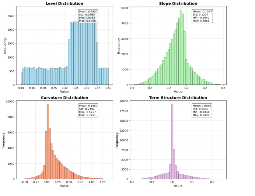
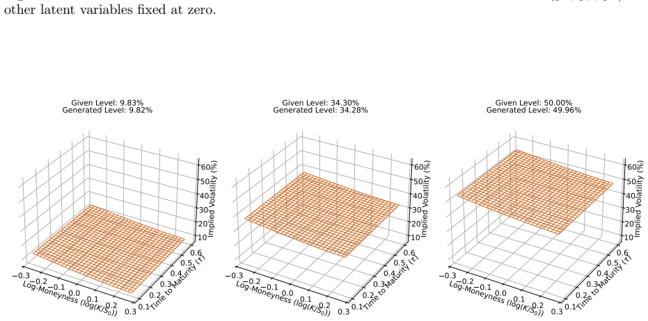
Central discovery: quantitative control of IVS shape and financial validity can live in one VAE. Four shape features (level, slope, curvature, term structure) are anchor-point derivatives estimated by bivariate polynomial regression and fed to the decoder as controllable latent variables. A post-generation step re-optimizes only the residual latent variables against calendar-spread and butterfly penalties, leaving commanded features untouched. Results: level-generation error below 0.1% in most trials; four-feature control keeps errors mostly below 10^-2 and renders residual latents nearly inert; all 60,000 in-distribution surfaces satisfy no-arbitrage conditions; about 45.5% of rare tail vio
Load-bearing premise
The four controlled 'shape features' are coefficients of a polynomial fitted to the surface on a grid whose shortest maturity is τ = 0.1 and then extrapolated to the anchor point τ → 0+, m = 0; if that extrapolation does not capture the economically meaningful limiting shape, hitting the coefficients precisely does not control the market-relevant surface.
Editorial extensions
If this is right
- Stress-test scenario design becomes a matter of dialing in feature values: surfaces with elevated volatility levels, steepened skews, or inverted term structures can be generated in a single decoder pass, without re-calibrating a pricing model.
- Surfaces sampled within the convex hull of the training feature space are, according to Section 5.3, observed to be free of calendar-spread and butterfly arbitrage in all 60,000 draws, so downstream pricing or hedging tasks can consume them directly.
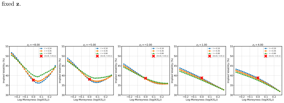
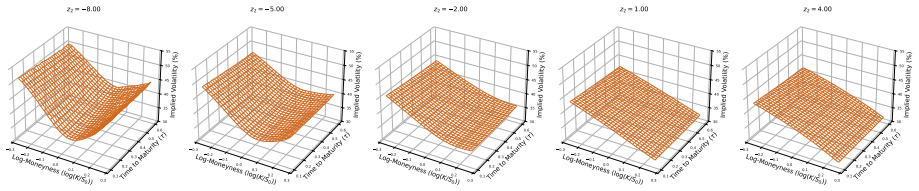
- When fewer than four features are controlled, the residual latent variables still carry meaningful structure (z2 correlates with slope at about -0.991 in the single-feature experiment), so the model doubles as an exploratory tool for finding stylized facts the user did not specify.
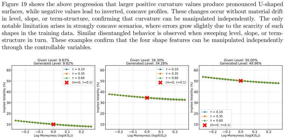
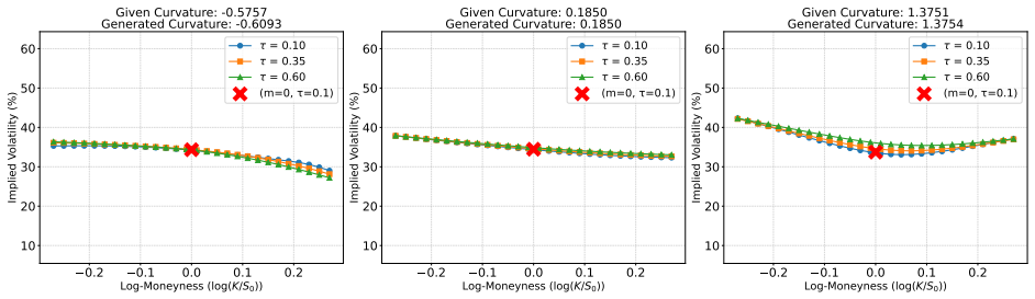
- When all four stylized factors are supervised, the residual latent variables become nearly inert (feature fluctuations on the order of 10^-3 across an eight-standard-deviation sweep), meaning the four-feature model gives essentially complete control over the dominant modes of IVS variation.
- Extreme latent draws can produce slope values beyond the training range, so the generator can extrapolate to market states — steep skews or inverted term structures — that are rare or absent in the training data.
Reading between the lines
- The same split-latent recipe should transfer wherever a high-dimensional market object is summarized by a handful of interpretable coefficients — for instance implied correlation surfaces, variance swap term structures, or CDS surfaces — since nothing in the architecture depends on equities except the choice of the four features.
- A natural upgrade the authors flag but do not pursue: replace the polynomial basis with functions that can represent the exploding ATM slope of short-expiry surfaces, as in rough-volatility models. Until then, 'slope' means the polynomial's slope on the τ ≥ 0.1 grid extrapolated to τ = 0, and that extrapolation deserves validation against true short-time asymptotics before the control variable is
- The repair algorithm keeps y fixed by construction but can push z away from the Gaussian prior; checking the posterior density of repaired z's and re-testing arbitrage after a second repair cycle would clarify whether the 45.5% correction rate is a property of the decoder or an artifact of L-BFGS initialization, which the paper itself flags as a local-optimization procedure.
- For deployment, the convex-hull result suggests a cheap safety wrapper: constrain each sampled y to the training feature hull (a few linear inequality checks) and z to the central region, and arbitrage violations should effectively never occur — trading a little diversity for a certificate of validity.
Editorial analysis
A structured set of objections, weighed in public.
Referee Report
Summary. The paper proposes a controllable VAE for generating implied volatility surfaces (IVSs) with user-specified shape features. Four features (level, slope, curvature, term-structure slope) are quantified as coefficients of a bivariate polynomial regression evaluated at an anchor point (τ→0, m=0). These features serve as controllable variables y, while residual latent variables z capture remaining variability; training uses a conditional VAE objective with a β-weighted KL term. Experiments on 60,000 synthetic Heston/SABR surfaces report low generation errors in single- and multi-feature control, latent-traversal diversity, and no-arbitrage checks with a post-generation latent-space repair algorithm.
Significance. If the central claims hold, the framework would be a practically useful tool for stress testing and scenario generation, combining interpretable financial features with deep generative modeling. The paper contains a clean derivation of the conditional VAE ELBO (Appendix C), tests on two stochastic-volatility model families, and explicit no-arbitrage validation on generated surfaces. However, the evidence for the main claim of 'precise controllability' is weakened by two intertwined issues: the anchor-point features are extrapolated far outside the data support, and the evaluation applies the same regression operator that defines the conditioning labels to the generated surfaces. These issues make the reported sub-0.1% errors partly self-referential and not yet established as control of market-relevant surface shape.
major comments (4)
- [§3.3, Eq. (33), and Appendix B] The four controlled features are regression coefficients fitted on τ∈[0.1,0.6] and m∈[−0.27,0.27] but evaluated at the anchor point (τ=0, m=0). In particular, Σ1,0 is the τ-derivative at τ=0 estimated from a polynomial fit far from the origin, and the Remark after Eq. (12) acknowledges that the regression cannot capture singular short-end slopes. Since the data grid does not include τ near 0, the features are extrapolations, not interpolations. The sub-0.1% errors in §5.1.1 therefore establish control over polynomial coefficients, not necessarily over economically meaningful surface shape. The paper should provide a stability analysis with respect to the polynomial orders J,L(J) (which are never stated) and validate control errors using features measured on the observed grid, e.g., at the shortest maturity τ=0.1.
- [§5.1.1 and Eq. (10)] The generation error is computed by applying the same differential operator P (Eqs. 9–12) that defines the conditioning labels y(given) to the generated surface to obtain y(generated). The decoder is trained with labels extracted via this same operator (Section 4.3). Low |e| thus partly reflects how well the decoder inverts P on the training manifold, rather than how well the generated IVS matches an independently defined shape target. This closed loop does not invalidate the method, but it means the headline 'control accuracy' is not yet evidence of control over the underlying surface geometry. Please add an independent evaluation, e.g., fit SVI or a different parametric form to generated surfaces and compare those parameters, or measure features by finite differences at the shortest available maturity.
- [§5.3, Table 3] The post-generation repair algorithm fixes only 45.5% of the violating surfaces, leaving 2,950 of 60,000 generated samples (4.9%) in violation of static no-arbitrage conditions. The text concludes that the method 'can be corrected effectively' and that violations 'remain rare and can be corrected effectively'; given that over half of the violations are unrepaired, this is an overstatement. Moreover, Algorithm 2 optimizes z while keeping y fixed, but the decoded repaired surface may still have a different measured y, and LMSE only constrains the surface deviation, not the feature deviation. Please report the distribution of y errors before and after repair, and discuss the residual 4.9% violation rate.
- [§5 (all experiments)] The paper repeatedly contrasts the framework with 'black-box generators' and claims that it 'combines interpretability, controllability, and flexibility', but no baseline comparisons are provided. Without comparisons to, e.g., a conditional VAE that conditions on raw grid points or on PCA scores, a linear decoder-plus-regression model, or an existing IVS GAN, the experimental section cannot support the relative advantages asserted in the introduction and conclusion. At minimum, report control error and arbitrage-violation rates for a simple conditional VAE or a regression-based generator on the same dataset.
minor comments (6)
- [§3.3 / Appendix B] The polynomial orders J and L(J) in Eq. (33) are never specified, and no sensitivity study is reported. Since these orders define the feature values, the reader cannot reproduce the experiments or assess the stability of the anchor-point extrapolation.
- [§5.2 / Table 1] The KL weight β is listed as 'problem-specific' but only the three-feature experiment states a value (β=5×10^-8). Please report β for the single- and four-feature experiments, and describe how it was selected.
- [§4.4 / Algorithm 2] The thresholds ε1, ε2, maximum iterations T, and the learning rate η in Algorithm 2 are not given numerically, and no convergence statistics are reported. Please provide the implementation values or a reference to released code.
- [§5.1.3] The latent traversal uses z2=±8, which is 8 standard deviations under the standard normal prior and has negligible prior probability. The claim that the model 'can extrapolate meaningfully' would be stronger if these out-of-distribution surfaces were also checked for no-arbitrage violations and compared with in-distribution latent samples.
- [Figures 11 and 16] The legend entries in Figures 11 and 16 appear as 'uni000000/...' encoding artifacts rather than readable feature names; these should be fixed.
- [§1 and §5.1.1] Typos and minor wording: 'A serial of studies' should be 'A series of studies'; in Section 5.1.1, the sentence beginning 'whered y(given)L' has a stray 'd'.
Circularity Check
Control metric is closed-loop: generation error is measured with the same regression operator P that defines the controllable labels, so sub-0.1% accuracy partly restates decoder inversion of P.
-
self definitional
[Section 5.1.1 (Overall Performance), referencing Section 3.3 Eqs. (9)-(12)]
"For each case, we define the generation error eL = y(generated)L − y(given)L , where y(given)L stands for the desired level which is given to the input of the generator (i.e., the already trained decoder), and y(generated)L stands for the volatility level of a generated IVS, which is computed using the regression method in Section 3.3."
The controllable labels y are extracted by the regression operator P (Eq. 10: yi = Pg(τ,m|xi)), whose coefficients define the very 'shape features' that the paper claims to control. The success metric then computes y(generated) by applying the same operator P to the decoded surface. Consequently, the reported sub-0.1% generation error measures how well the decoder inverts P on user-supplied labels (P∘Decoder ≈ Id) rather than providing an independent check that economically meaningful surface shape has been controlled. Moreover, because y is a deterministic function of the training surface x and the decoder is trained to reconstruct x under an MSE loss (Eq. 45), matching y is largely inherited from the reconstruction objective, making the 'precise controllability' claim partly a restatemen
full rationale
The paper does not rely on load-bearing self-citations: the anchor-point regression method is attributed to external work ([27],[34]) and the VAE machinery is standard. The central architecture—explicit controllable y, residual latent z, and post-generation arbitrage repair—is independently implemented and tested against no-arbitrage conditions that are not derived from the feature operator. The main circularity concern is the evaluation protocol: the features that define the control targets are the same regression coefficients used to measure generation success. Thus the quantitative controllability results are self-referential: they demonstrate that the decoder can invert the feature-extraction map, not that the underlying polynomial coefficients correspond to robust, economically meaningful shape attributes. The paper itself acknowledges a limitation in the Remark after Eq. (12) that the regression cannot capture singular short-end slopes, which is exactly the regime where the anchor-point extrapolation (from τ∈[0.1,0.6] to τ→0+) is most fragile. That extrapolation instability is a correctness risk rather than circularity. Overall, the circularity is partial: the framework has independent content, but the headline 'precise control' metric is closed-loop and should be interpreted as control over the regression-defined features, not as an externally validated control of surface shape.
Assumptions & free parameters
free parameters (4)
- beta (KL weight) =
5e-8 (three-feature); problem-specific in Table 1
- latent dimension =
5
- polynomial regression orders J, L(J) =
not reported
- Algorithm 2 thresholds and max iterations =
not reported
assumptions (4)
- standard math Implied volatility is uniquely defined by inverting the Black-Scholes formula.
- domain assumption The no-arbitrage conditions, expressed via total variance w = sigma^2 tau, are those of Gatheral-Jacquier (calendar and butterfly).
- domain assumption The IVS can be represented by a bivariate polynomial around the anchor point, and the limiting Taylor coefficients exist and are finite.
- ad hoc to paper The joint distribution factorizes as p(x,y,z)=p(z)p(y)p(x|y,z) with independent y and z.
Cite this review
Pith. "Pith review of Controllable Generation of Implied Volatility Surfaces with Variational Autoencoders." pith.science (2026). https://pith.science/paper/PKUCUQUP
@misc{pith2026250901743,
  author       = {Pith},
  title        = {Pith review of: Controllable Generation of Implied Volatility Surfaces with Variational Autoencoders},
  year         = {2026},
  howpublished = {\url{https://pith.science/paper/PKUCUQUP}},
  note         = {Machine review of arXiv:2509.01743}
}
read the original abstract
This paper presents a deep generative modeling framework for controllably synthesizing implied volatility surfaces (IVSs) using a variational autoencoder (VAE). Unlike conventional data-driven models, our approach provides explicit control over meaningful shape features (e.g., volatility level, slope, curvature, term-structure) to generate IVSs with desired characteristics. In our framework, financially interpretable shape features are disentangled from residual latent factors. The target features are embedded into the VAE architecture as controllable latent variables, while the residual latent variables capture additional structure to preserve IVS shape diversity. To enable this control, IVS feature values are quantified via regression at an anchor point and incorporated into the decoder to steer generation. Numerical experiments demonstrate that the generative model enables rapid generation of realistic IVSs with desired features rather than arbitrary patterns, and achieves high accuracy across both single- and multi-feature control settings. For market validity, an optional post-generation latent-space repair algorithm adjusts only the residual latent variables to remove occasional violations of static no-arbitrage conditions without altering the specified features. Compared with black-box generators, the framework combines interpretability, controllability, and flexibility for synthetic IVS generation and scenario design.
Figures


Figures from the paper (32 more)










Forward citations
Cited by 1 Pith paper
-
Latent Flow Matching for Arbitrage-Aware Implied Volatility Surface Generation
Latent flow matching with an arbitrage-regularized VAE generates implied volatility surfaces that match the empirical distribution and pass static no-arbitrage tests at a higher rate than GAN and diffusion baselines.
Reference graph
Works this paper leans on
- [1]
-
[2]
Practical guide to economic scenario generators
Society of Actuaries. Practical guide to economic scenario generators. Soa research report, Society of Actuaries, 2016. 24
work page 2016
-
[3]
Regulation (eu) no 575/2013 of the european parliament and of the council on prudential require- ments for credit institutions and investment firms (capital requirements regulation). https://eur-lex. europa.eu/legal-content/EN/TXT/?uri=CELEX%3A02013R0575-20240709, 2013. Accessed: 2025-08- 13
work page 2013
-
[4]
Financial crises, implied volatility and stress testing
Allan M Malz. Financial crises, implied volatility and stress testing. Riskmetrics group, New York , 2001
work page 2001
-
[5]
Hans Buehler, Lukas Gonon, Josef Teichmann, and Ben Wood. Deep hedging. Quantitative Finance, 19(8):1271–1291, 2019
work page 2019
-
[6]
Steven L Heston. A closed-form solution for options with stochastic volatility with applications to bond and currency options. The review of financial studies , 6(2):327–343, 1993
work page 1993
-
[7]
Pricing under rough volatility
Christian Bayer, Peter Friz, and Jim Gatheral. Pricing under rough volatility. Quantitative Finance , 16(6):887–904, 2016
work page 2016
-
[8]
Arbitrage-free svi volatility surfaces
Jim Gatheral and Antoine Jacquier. Arbitrage-free svi volatility surfaces. Quantitative Finance , 14(1):59–71, 2014
work page 2014
Show all 48 references
-
[9]
Pricing with a smile
Bruno Dupire et al. Pricing with a smile. Risk, 7(1):18–20, 1994
1994
-
[10]
Generative models in finance: Market generators, a paradigm shift in financial modeling
Blanka Horvath, Jonathan Plenk, Milena Vuleti´ c, and Raeid Saqur. Generative models in finance: Market generators, a paradigm shift in financial modeling. https://ssrn.com/abstract=5284313, June 2025. Available at SSRN: https://ssrn.com/abstract=5284313 or http://dx.doi.org/1...
2025
-
[11]
Gaussian genai: Synthetic market data generation
Joerg Kienitz. Gaussian genai: Synthetic market data generation. Risk, 2025
2025
-
[12]
Simulation of arbitrage-free implied volatility surfaces
Rama Cont and Milena Vuleti´ c. Simulation of arbitrage-free implied volatility surfaces. Applied Math- ematical Finance, 30(2):94–121, 2023
2023
-
[13]
Kingma, Shakir Mohamed, Danilo Jimenez Rezende, and Max Welling
Diederik P. Kingma, Shakir Mohamed, Danilo Jimenez Rezende, and Max Welling. Semi-supervised learning with deep generative models. Advances in neural information processing systems , 27, 2014
2014
-
[14]
Generative adversarial nets
Ian J Goodfellow, Jean Pouget-Abadie, Mehdi Mirza, Bing Xu, David Warde-Farley, Sherjil Ozair, Aaron Courville, and Yoshua Bengio. Generative adversarial nets. Advances in neural information processing systems, 27, 2014
2014
-
[15]
Denoising diffusion probabilistic models
Jonathan Ho, Ajay Jain, and Pieter Abbeel. Denoising diffusion probabilistic models. Advances in neural information processing systems , 33:6840–6851, 2020
2020
-
[16]
Volgan: A generative model for arbitrage-free implied volatility surfaces
Milena Vuleti´ c and Rama Cont. Volgan: A generative model for arbitrage-free implied volatility surfaces. Applied Mathematical Finance, 31(4):203–238, 2024
2024
-
[17]
Computing volatility surfaces using generative adversarial networks with minimal arbitrage violations, 2023
Andrew Na, Meixin Zhang, and Justin Wan. Computing volatility surfaces using generative adversarial networks with minimal arbitrage violations, 2023
2023
-
[18]
Variational autoen- coders: A hands-off approach to volatility
Maxime Bergeron, Nicholas Fung, John Hull, Zissis Poulos, and Andreas Veneris. Variational autoen- coders: A hands-off approach to volatility. arXiv preprint arXiv:2102.03945 , 2021
2021 arXiv
-
[19]
Arbitrage-free implied volatility surface generation with variational autoencoders
Brian (Xin) Ning, Sebastian Jaimungal, Xiaorong Zhang, and Maxime Bergeron. Arbitrage-free implied volatility surface generation with variational autoencoders. SIAM Journal on Financial Mathematics , 14(4):1004–1027, 2023
2023
-
[20]
Deep weighted monte carlo: a hybrid option pricing framework using neural networks
S´ andor Kuns´ agi-M´ at´ e, G´ abor F´ ath, Istv´ an Csabai, and G´ abor Moln´ ar-S´ aska. Deep weighted monte carlo: a hybrid option pricing framework using neural networks. Quantitative Finance, 23(4):615–629, 2023
2023
-
[21]
Filling in missing FX implied volatilities with uncertainties: Improving V AE-based volatility imputation
Achintya Gopal. Filling in missing FX implied volatilities with uncertainties: Improving V AE-based volatility imputation. arXiv preprint arXiv:2411.05998 , 2024. 25
2024 arXiv
-
[22]
β-V AE: Learning basic visual concepts with a constrained varia- tional framework
Irina Higgins, Loic Matthey, Arka Pal, Christopher Burgess, Xavier Glorot, Matthew Botvinick, Shakir Mohamed, and Alexander Lerchner. β-V AE: Learning basic visual concepts with a constrained varia- tional framework. In International conference on learning representations , 2017
2017
-
[23]
Dynamics of implied volatility surfaces
Rama Cont and J´ ulio da Fonseca. Dynamics of implied volatility surfaces. Quantitative Finance , 2(1):45–60, 2002
2002
-
[24]
Venturing into uncharted territory: An extensible implied volatility surface model
Pascal Fran¸ cois, R´ emi Galarneau-Vincent, Genevi` eve Gauthier, and Fr´ ed´ eric Godin. Venturing into uncharted territory: An extensible implied volatility surface model. Journal of Futures Markets , 42(10):1912–1940, 2022
1912
-
[25]
The supply and demand of s&p 500 put options
George M Constantinides and Lei Lian. The supply and demand of s&p 500 put options. Technical report, National Bureau of Economic Research, 2015
2015
-
[26]
What type of process underlies options? a simple robust test
Peter Carr and Liuren Wu. What type of process underlies options? a simple robust test. The Journal of Finance, 58(6):2581–2610, 2003
2003
-
[27]
Implied stochastic volatility models
Yacine A ¨ ıt-Sahalia, Chenxu Li, and Chen Xu Li. Implied stochastic volatility models. The Review of Financial Studies , 34(1):394–450, 2021
2021
-
[28]
Tsekrekos
Georgios Chalamandaris and Andrianos E. Tsekrekos. How important is the term structure in implied volatility surface modeling? evidence from foreign exchange options. Journal of International Money and Finance, 30(4):623–640, 2011
2011
-
[29]
Pricing event risk: Evidence from concave implied volatility curves
Lykourgos Alexiou, Amit Goyal, Alexandros Kostakis, and Leonidas Rompolis. Pricing event risk: Evidence from concave implied volatility curves. Review of Finance , page rfaf016, 2025
2025
-
[30]
The Volatility Surface: A Practitioner’s Guide
Jim Gatheral. The Volatility Surface: A Practitioner’s Guide . John Wiley & Sons, 2006
2006
-
[31]
Does net buying pressure affect the shape of implied volatility functions? Journal of Finance , 59(2):711–753, 2004
Nicolas PB Bollen and Robert E Whaley. Does net buying pressure affect the shape of implied volatility functions? Journal of Finance , 59(2):711–753, 2004
2004
-
[32]
Roger W. Lee. The moment formula for implied volatility at extreme strikes. Mathematical Finance, 12(4):469–480, 2002
2002
-
[33]
The term structure of variance swap rates and optimal variance swap investments
Daniel Egloff, Markus Leippold, and Liuren Wu. The term structure of variance swap rates and optimal variance swap investments. Journal of Finance , 65(2):721–759, 2010
2010
-
[34]
Malliavin calculus in finance: Theory and practice
Elisa Al` os and David Garcia Lorite. Malliavin calculus in finance: Theory and practice . Chapman and Hall/CRC, 2021
2021
-
[35]
Closed-form implied volatility surfaces for stochastic volatility models with jumps
Yacine A ¨ ıt-Sahalia, Chenxu Li, and Chen Xu Li. Closed-form implied volatility surfaces for stochastic volatility models with jumps. Journal of Econometrics , 222(1, Part B):364–392, 2021
2021
-
[36]
Disentangled variational auto-encoder for semi-supervised learning
Yang Li, Quan Pan, Suhang Wang, Haiyun Peng, Tao Yang, and Erik Cambria. Disentangled variational auto-encoder for semi-supervised learning. Information Sciences, 482:73–85, 2019
2019
-
[37]
Capturing label character- istics in V AEs
Tom Joy, Sebastian Schmon, Philip Torr, N Siddharth, and Tom Rainforth. Capturing label character- istics in V AEs. In International Conference on Learning Representations , 2021
2021
-
[38]
Learning disentangled representations with semi-supervised deep generative models
Brooks Paige, Jan-Willem Van De Meent, Alban Desmaison, Noah Goodman, Pushmeet Kohli, Frank Wood, Philip Torr, et al. Learning disentangled representations with semi-supervised deep generative models. Advances in neural information processing systems , 30, 2017
2017
-
[39]
Deep residual learning for image recognition
Kaiming He, Xiangyu Zhang, Shaoqing Ren, and Jian Sun. Deep residual learning for image recognition. In 2016 IEEE Conference on Computer Vision and Pattern Recognition (CVPR) , pages 770–778, 2016
2016
-
[40]
Liu and Jorge Nocedal
Dong C. Liu and Jorge Nocedal. On the limited memory bfgs method for large scale optimization. Mathematical Programming, 45(1–3):503–528, 1989. 26
1989
-
[41]
Cox, Jonathan E
John C. Cox, Jonathan E. Ingersoll, and Stephen A. Ross. A theory of the term structure of interest rates. Econometrica, 53(2):385–407, 1985
1985
-
[42]
Oosterlee
Fang Fang and Cornelis W. Oosterlee. A novel pricing method for european options based on fourier- cosine series expansions. SIAM Journal on Scientific Computing , 31(2):826–848, 2009
2009
-
[43]
Mathematical modeling and computation in finance: with exercises and Python and MATLAB computer codes
Cornelis W Oosterlee and Lech A Grzelak. Mathematical modeling and computation in finance: with exercises and Python and MATLAB computer codes . World Scientific, 2019
2019
-
[44]
Blei, Alp Kucukelbir, and Jon D
David M. Blei, Alp Kucukelbir, and Jon D. McAuliffe. Variational inference: A review for statisticians. Journal of the American Statistical Association , 112(518):859–877, 2017
2017
-
[45]
Kingma and Max Welling
Diederik P. Kingma and Max Welling. Auto-encoding variational Bayes.arXiv preprint arXiv:1312.6114, 2013. A Training dataset The dataset used to train the V AE consists of 60,000 IVSs, synthesized from 30,000 Heston and 30,000 SABR samples. The distribution of features of the ...
2013 arXiv
-
[46]
(33) Here, J ∈ N and L(J) = (L0, L1,
We first express the IVS locally using a bivariate Taylor expansion around the anchor point: x(J,L(J))(τ, m) = JX j=0 LjX i=0 β(i,j)τ imj, where β(i,j) = Σi,j i! j! . (33) Here, J ∈ N and L(J) = (L0, L1, . . . , LJ ) are finite expansion orders in each direction. 30
-
[47]
Given a dataset consisting of n daily IVSs, we fit the expansion in Equation (33) via polynomial regression on each day l = 1, . . . , n. The observed IVS values xdata(τ (s) l , m(s) l ) are approximated as: xdata(τ (s) l , m(s) l ) = JX j=0 LjX i=0 β(i,j) l (τ (s) l )i(m(s) l...
-
[48]
term-structure
Finally, the estimated shape characteristics on day l are recovered as: [Σi,j]data l = i! j! ˆβ(i,j) l , for i, j≥ 0. (35) C Derivation of conditional V AE A central task in training generative models is to estimate the model parameters θ such that the resulting distribution p...
Reviewed August 5, 2026 · model on record in the stance chip above.
Discussion (0). Continue with ORCID to comment.