Inference on covariance structure in high-dimensional multi-view data
Pith reviewed 2026-05-18 19:03 UTC · model grok-4.3
The pith
Spectral decompositions align latent factors in multi-view data so that conjugate priors produce closed-form posteriors for high-dimensional covariance estimation.
A machine-rendered reading of the paper's core claim, the machinery that carries it, and where it could break.
Core claim
Conditionally on latent factors recovered by spectral decomposition, jointly conjugate priors for factor loadings and residual variances yield a posterior that is exactly a product of normal-inverse-gamma distributions across variables; the resulting procedure therefore admits direct posterior sampling and satisfies increasing-dimension posterior contraction together with central limit theorems for point estimators.
What carries the argument
Spectral decomposition that estimates and aligns latent factors active in at least one view, which then conditions the choice of jointly conjugate priors for loadings and variances to obtain the product posterior.
If this is right
- Posterior computation reduces to direct sampling from independent normal-inverse-gamma distributions for each variable.
- Uncertainty quantification remains accurate rather than underestimated by variational approximations.
- Point estimators obey central limit theorems, permitting standard-error-based inference in high dimensions.
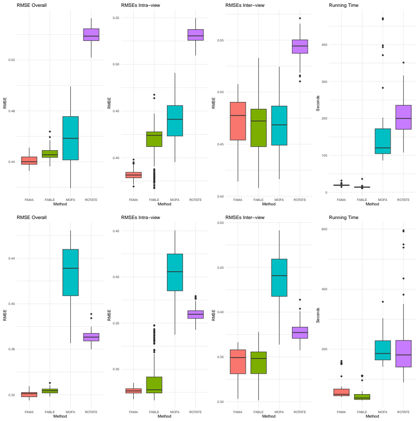
- The procedure scales to integrating four or more high-dimensional views, as demonstrated on multi-omics cancer data.
Where Pith is reading between the lines
- The same spectral-plus-conjugate construction could be tested on single-view factor models if the alignment step is replaced by a suitable initialization.
- Robustness checks could examine performance when some latent factors are weak or when views have mismatched sample sizes.
- The closed-form posterior might be combined with variable selection penalties to produce sparse multi-view covariance estimates.
Load-bearing premise
Spectral decompositions can reliably recover and align the latent factors that are active in at least one view from the observed multi-view data.
What would settle it
A simulation or real dataset in which the spectral estimates fail to align the active factors and the resulting posterior intervals or point estimators do not contract at the claimed rate.
Figures


read the original abstract
This article focuses on covariance estimation for multi-view data. Popular approaches rely on factor-analytic decompositions that have shared and view-specific latent factors. Posterior computation is conducted via expensive and brittle Markov chain Monte Carlo (MCMC) sampling or variational approximations that underestimate uncertainty and lack theoretical guarantees. Our proposed methodology employs spectral decompositions to estimate and align latent factors that are active in at least one view. Conditionally on these factors, we choose jointly conjugate prior distributions for factor loadings and residual variances. The resulting posterior is a simple product of normal-inverse gamma distributions for each variable, bypassing MCMC and facilitating posterior computation. We prove favorable increasing-dimension asymptotic properties, including posterior contraction and central limit theorems for point estimators. We show excellent performance in simulations, including accurate uncertainty quantification, and apply the methodology to integrate four high-dimensional views from a multi-omics dataset of cancer cell samples.
Editorial analysis
A structured set of objections, weighed in public.
Referee Report
Summary. The paper develops a covariance estimation procedure for high-dimensional multi-view data. Latent factors shared or active across views are estimated and aligned via spectral decomposition. Conditionally on these point estimates, jointly conjugate normal-inverse-gamma priors are placed on loadings and residual variances, yielding an exact product-of-NIG posterior that avoids MCMC. The authors establish increasing-dimension posterior contraction and central limit theorems for the resulting point estimators, demonstrate accurate uncertainty quantification in simulations, and apply the method to a four-view multi-omics cancer dataset.
Significance. If the central claims hold, the work supplies a computationally tractable, theoretically supported alternative to MCMC or variational methods for multi-view covariance inference. The closed-form posterior factorization and the increasing-dimension contraction/CLT results are substantive strengths; the simulation performance and multi-omics application further indicate practical utility for high-dimensional integrative analyses.
major comments (2)
- [§4] §4 (asymptotic theory): The posterior contraction and CLT statements are derived conditionally on the spectrally estimated factors. To transfer these guarantees to the unconditional procedure, uniform bounds on the spectral estimation error (in operator or Frobenius norm) that are o_p of the target contraction rate are required when both dimension p and the number of views grow; the manuscript does not appear to supply such bounds, leaving open whether the plug-in step preserves the stated rates or only approximates them.
- [§3.2] §3.2 (posterior construction): The claim that the posterior is exactly a product of normal-inverse-gamma distributions relies on treating the spectral factor estimates as fixed. Because the factor estimates are data-dependent, the joint posterior for loadings and variances is no longer exactly conjugate with respect to the original data-generating measure; an explicit error-propagation argument or marginalization step would be needed to justify the exact factorization used for uncertainty quantification.
minor comments (2)
- [§2] Notation for the number of views and the alignment step across views should be introduced earlier and used consistently in the model statement.
- [Figure 1] Figure 1 (simulation results): axis labels and legend entries are too small for readability; consider increasing font size or splitting into two panels.
Simulated Author's Rebuttal
We thank the referee for their thorough review and valuable suggestions. We address each major comment below and outline the revisions we will make to strengthen the manuscript.
read point-by-point responses
-
Referee: [§4] §4 (asymptotic theory): The posterior contraction and CLT statements are derived conditionally on the spectrally estimated factors. To transfer these guarantees to the unconditional procedure, uniform bounds on the spectral estimation error (in operator or Frobenius norm) that are o_p of the target contraction rate are required when both dimension p and the number of views grow; the manuscript does not appear to supply such bounds, leaving open whether the plug-in step preserves the stated rates or only approximates them.
Authors: We agree with the referee that the current asymptotic results are conditional on the factor estimates obtained via spectral decomposition. In the revised manuscript, we will add a new subsection in §4 providing uniform bounds on the spectral estimation error in the operator norm. Under the assumptions of the factor model and with appropriate growth rates for p and the number of views, we show that this error is of smaller order than the posterior contraction rate, thereby transferring the guarantees to the unconditional procedure. This will be supported by additional lemmas on the concentration of the spectral estimators. revision: yes
-
Referee: [§3.2] §3.2 (posterior construction): The claim that the posterior is exactly a product of normal-inverse-gamma distributions relies on treating the spectral factor estimates as fixed. Because the factor estimates are data-dependent, the joint posterior for loadings and variances is no longer exactly conjugate with respect to the original data-generating measure; an explicit error-propagation argument or marginalization step would be needed to justify the exact factorization used for uncertainty quantification.
Authors: The referee correctly notes that the exact conjugacy and product-of-NIG form holds conditionally on the fixed factor estimates. We will revise the text in §3.2 to clarify this conditional nature explicitly. Additionally, we will include an error-propagation argument demonstrating that the total variation distance or other discrepancy between the conditional posterior and the true joint posterior vanishes asymptotically at the rates established in §4. This justifies the use of the conditional posterior for practical uncertainty quantification in high dimensions. revision: yes
Circularity Check
No significant circularity; posterior follows from standard conjugate update conditional on external spectral estimates
full rationale
The derivation estimates latent factors via spectral decomposition of the observed data, then conditions on those point estimates to select jointly conjugate priors for loadings and variances. The resulting posterior is obtained by direct application of Bayes' rule under the conditional model, producing the claimed product of normal-inverse-gamma distributions. This is a standard, non-circular construction. The increasing-dimension posterior contraction and CLT results are established via separate asymptotic analysis under stated assumptions on the factor estimates; they do not reduce to redefinitions or self-citations of the target quantities. The method is self-contained against external benchmarks once the spectral step is accepted as a fixed input.
Axiom & Free-Parameter Ledger
axioms (1)
- domain assumption The observed multi-view data arise from a factor model containing both shared and view-specific latent factors.
Lean theorems connected to this paper
-
IndisputableMonolith/Foundation/RealityFromDistinction.leanreality_from_one_distinction unclear?
unclearRelation between the paper passage and the cited Recognition theorem.
employs spectral decompositions to estimate and align latent factors... resulting posterior is a simple product of normal-inverse gamma distributions... prove favorable increasing-dimension asymptotic properties, including posterior contraction and central limit theorems
-
IndisputableMonolith/Cost/FunctionalEquation.leanwashburn_uniqueness_aczel unclear?
unclearRelation between the paper passage and the cited Recognition theorem.
JIC-based selection of latent dimensions and variance-inflation tuning for frequentist coverage
What do these tags mean?
- matches
- The paper's claim is directly supported by a theorem in the formal canon.
- supports
- The theorem supports part of the paper's argument, but the paper may add assumptions or extra steps.
- extends
- The paper goes beyond the formal theorem; the theorem is a base layer rather than the whole result.
- uses
- The paper appears to rely on the theorem as machinery.
- contradicts
- The paper's claim conflicts with a theorem or certificate in the canon.
- unclear
- Pith found a possible connection, but the passage is too broad, indirect, or ambiguous to say the theorem truly supports the claim.
Reference graph
Works this paper leans on
-
[1]
Akbani, R., Ng, P. K. S., Werner, H. M. J. & et al. (2014), ‘A pan-cancer proteomic perspective on The Cancer Genome Atlas’,Nature Communications 5,
work page 2014
-
[2]
URL: https://doi.org/10.1038/ncomms4887 Anastasiadi, D., Esteve-Codina, A. & Piferrer, F. (2018), ‘Consistent inverse correlation between DNA methylation of the first intron and gene expression across tissues and species’,Epigenetics & Chromatin 11(1),
-
[3]
URL: https://doi.org/10.1186/s13072-018-0205-1 Anceschi, N., Ferrari, F., Dunson, D. B. & Mallick, H. (2024), ‘Bayesian joint additive factor models for multiview learning’,arXiv preprint arXiv:2406.00778 . Argelaguet, R., Arnol, D., Bredikhin, D., Deloro, Y., Velten, B., Marioni, J. & Stegle, O. (2020), ‘MOFA+: A statistical framework for comprehensive i...
-
[4]
Argelaguet, R., Velten, B., Arnol, D., Dietrich, S., Zenz, T., Marioni, J. C., Buettner, F., Huber, W. & Stegle, O. (2018), ‘Multi-omics factor analysis—a framework for unsupervised integration of multi-omics data sets’,Molecular Systems Biology 14(6), e8124. Bai, J. (2003), ‘Inferential theory for factor models of large dimensions’,Econometrica 71(1), 135–
work page 2018
-
[5]
18 Bandeira, A. S. & van Handel, R. (2016), ‘Sharp nonasymptotic bounds on the norm of random matrices with independent entries’,The Annals of Probability 44(4), 2479 –
work page 2016
-
[6]
Bhattacharya, A., Bense, R. D., Urz´ ua-Traslavi˜na, C. G. et al. (2020), ‘Transcriptional effects of copy number alterations in a large set of human cancers’,Nature Communications 11(1),
work page 2020
-
[7]
URL: https://doi.org/10.1038/s41467-020-14605-5 Chattopadhyay, S., Zhang, A. R. & Dunson, D. B. (2024), ‘Blessing of dimension in Bayesian inference on covariance matrices’,arXiv preprint arXiv:2404.03805 . Chen, Y. & Li, X. (2021), ‘Determining the number of factors in high-dimensional generalized latent factor models’,Biometrika 109(3), 769–782. Chen, Y...
-
[8]
Gratton, S. & Tshimanga-Ilunga, J. (2016), ‘On a second-order expansion of the truncated singular subspace decomposition’,Numerical Linear Algebra with Applications 23(3), 519–534. 19 Gry, M., Rimini, R., Str ¨omberg, S., Asplund, A., Pont ´en, F., Uhlen, M. & Nilsson, P. (2009), ‘Correlations between RNA and protein expression profiles in 23 human cell l...
work page 2016
-
[9]
(1976), Modern Factor Analysis, University of Chicago Press
Harman, H. (1976), Modern Factor Analysis, University of Chicago Press. Hoerl, A. E. & Kennard, R. W. (1970), ‘Ridge Regression: Biased Estimation for Nonorthogonal Problems’,Technometrics 12(1), 55–67. Hutchinson, L. (2017), ‘Aneuploidy and immune evasion — a biomarker of response’, Nature Reviews Clinical Oncology 14(3),
work page 1976
-
[10]
URL: https://doi.org/10.1038/nrclinonc.2017.23 Ishwaran, B. H., J. & Rao, S. (2005), ‘Spike and slab variable selection: Frequentist and bayesian strategies’,The Annals of Statistics 33, 730–773. URL: https://api.semanticscholar.org/CorpusID:9004248 Jia, G., Ramalingam, T. R., Heiden, J. V., Gao, X., DePianto, D., Morshead, K. B., Modrusan, Z., Ramamoorth...
-
[11]
Lee, S. M., Chen, Y. & Sit, T. (2024), ‘A latent variable approach to learning high-dimensional multivariate longitudinal data’,arXiv preprint arXiv:2405.15053 . Lock, E. F., Hoadley, K. A., Marron, J. S. & Nobel, A. B. (2013), ‘Joint and individual variation explained (JIVE) for integrated analysis of multiple data types’,The Annals of Applied Statistics...
-
[12]
Loh, C.-Y., Chai, J. Y., Tang, T. F., Wong, W. F., Sethi, G., Shanmugam, M. K., Chong, P. P. & Looi, C. Y. (2019), ‘The E-cadherin and N-cadherin switch in epithelial-to-mesenchymal transition: Signaling, therapeutic implications, and challenges’,Cells 8(10),
work page 2019
-
[13]
Ma, Z. & Ma, R. (2024), ‘Optimal estimation of shared singular subspaces across multiple noisy matrices’,arXiv preprint arXiv:2411.17054 . Mauri, L., Anceschi, N. & Dunson, D. B. (2025), ‘Spectral decomposition-assisted multi-study factor analysis’,arXiv preprint arXiv:2502.14600 . Mauri, L. & Dunson, D. B. (2025), ‘Factor pre-training in Bayesian multiva...
-
[14]
Inference on covariance structure in high- dimensional multi-view data
Zito, A. & Miller, J. W. (2024), ‘Compressive Bayesian non-negative matrix factorization for mutational signatures analysis’,arXiv preprint arXiv:2404.10974 . 21 Supplementary material for “Inference on covariance structure in high- dimensional multi-view data” A Preliminary results Proposition 1 (Adapted from Proposition 3.5 of Chattopadhyay et al. (2024...
-
[15]
The result follows from Proposition 3.5 of Chattopadhyay et al
Since 𝑈0𝑚 = ˜𝑈0𝑚𝑅 for some orthogonal matrix 𝑅, where ˜𝑈0𝑚 is the matrix of left singular vectors of 𝐹0𝑚Λ⊤ 0𝑚, we have 𝑈0𝑚𝑈⊤ 0𝑚 = ˜𝑈0𝑚 ˜𝑈⊤ 0𝑚. The result follows from Proposition 3.5 of Chattopadhyay et al. (2024). Proposition
work page 2024
-
[16]
Combining all of the above, we obtain 𝑠𝑘0 1 𝑀 𝑀∑︁ 𝑚=1 𝑃0𝑚 ≥ 1 𝑀 𝑠𝑘0 (𝐷0)2𝑑 −2 ≍ 1 𝑀 , with probability at least 1 − 𝑜(1), since by Corollary 5.35 in Vershynin (2012), we have 𝑠𝑘0 (𝐷0) =√𝑛 − O (𝑘0) and 𝑑 = √𝑛 + O (Í 𝑚 𝑘 𝑚) with probability at least 1 − 𝑜(1). 22 Therefore, denoting with 𝐸 = 1 𝑀 Í𝑀 𝑚=1 Δ𝑚, we have || 𝐸 || < 1/𝑀 with probability at least 1 − ...
work page 2012
-
[17]
we have min𝑅:𝑅⊤ 𝑅=𝐼𝑘0 ||𝑈 −𝑈0𝑅|| = ||𝑈 −𝑈0 ˆ𝑅|| ≲ 1 𝑛 + 1 𝑝min , with probability at least 1 − 𝑜(1), where ˆ𝑅 is the orthogonal matrix achieving the minimum of the quantity on the left hand side. Recalling that ˆ𝐹 = √𝑛𝑈 and letting ˜𝑅 = 𝑉0 ˆ𝑅, we have || ˆ𝐹 − 𝐹0 ˜𝑅|| = || √𝑛𝑈 − 𝑈0𝐷0 ˆ𝑅|| ≤ || √𝑛(𝑈 − 𝑈0 ˆ𝑅)|| + || √𝑛𝑈0 ˆ𝑅 − 𝑈0𝐷0 ˆ𝑅|| ≤ √𝑛 1 𝑛 + 1 𝑝min + ma...
work page 2012
-
[18]
Recall thatˆΛ𝑚 = 𝑌 ⊤ 𝑚𝑈√𝑛/(𝑛+ 𝜏−2 𝑚 )
We start by establishing consistency of point estimates. Recall thatˆΛ𝑚 = 𝑌 ⊤ 𝑚𝑈√𝑛/(𝑛+ 𝜏−2 𝑚 ). Let 𝑚, 𝑚′ ∈ { 1, . . . , 𝑀 }, not necessarily distinct, and 𝑔𝑚𝑚′ = 𝑛 (𝑛+𝜏 −2𝑚 ) (𝑛+𝜏 −2 𝑚′ ) then ˆΛ𝑚 ˆΛ⊤ 𝑚′ = 𝑔𝑚𝑚′𝑌 ⊤ 𝑚𝑈𝑈 ⊤𝑌𝑚′ = 𝑔𝑚𝑚′𝑌 ⊤ 𝑚𝑈0𝑈⊤ 0 𝑌𝑚′ + 𝑔𝑚𝑚′𝑌 ⊤ 𝑚 𝑈𝑈 ⊤ − 𝑈0𝑈⊤ 0 𝑌𝑚′ and 𝑛 (𝑛 + 𝜏−2𝑚 )2 𝑌𝑚𝑈0𝑈⊤ 0 𝑌𝑚′ = 𝑛 (𝑛 + 𝜏−2𝑚 )2 𝐹0 𝐴𝑚Λ⊤ 0𝑚 + 𝐸𝑚 ⊤𝑈0𝑈⊤ 0 𝐹0 𝐴𝑚′ Λ...
work page 2012
-
[19]
In addition, with probability at least 1 − 𝑜(1), we have || 𝐸 ⊤ 𝑚𝐹0𝑚′ Λ⊤ 0𝑚′ || ≲ (√𝑛 + √𝑝𝑚)√𝑛𝑝 𝑚′ , || 𝐸 ⊤ 𝑚′ 𝐹0𝑚Λ⊤ 0𝑚|| ≲ (√𝑛 + √𝑝𝑚′ )√𝑛𝑝 𝑚 and || 𝐸 ⊤ 𝑚𝑈0𝑈⊤ 0 𝐸𝑚′ || ≲ (√𝑛 + √𝑝𝑚) (√𝑛 + √𝑝𝑚′ ) since || 𝐸𝑚|| ≲ √𝑛 + √𝑝𝑚, || 𝐸𝑚′ || ≲ √𝑛 + √𝑝𝑚′ || 𝐹0𝑚|| ≍ || 𝐹0𝑚′ || ≲ √𝑛, with probability at least 1 − 𝑜(1), by Lemma 4 and Corollary 5.35 of Vershynin (2012), ...
work page 2012
-
[20]
Recall ˆ𝜆𝑙 𝑗 = √𝑛 𝑛+𝜏 −2 𝑙 𝑈⊤𝑦 ( 𝑗 ) 𝑙 , where 𝑦 ( 𝑗 ) 𝑙 denotes the 𝑗-th column of 𝑌𝑙. Thus, ˆ𝜆⊤ 𝑚 𝑗 ˆ𝜆𝑚′ 𝑗′ = 𝑔𝑚𝑚′ 𝑦 ( 𝑗 )⊤ 𝑚 𝑈𝑈 ⊤𝑦 ( 𝑗′ ) 𝑚′ = 𝑔𝑚𝑚′ 𝑦 ( 𝑗 )⊤ 𝑚 𝑈0𝑈⊤ 0 𝑦 ( 𝑗′ ) 𝑚′ + 𝑔𝑚𝑚′ 𝑦 ( 𝑗 )⊤ 𝑚 𝑈𝑈 ⊤ − 𝑈0𝑈⊤ 0 𝑦 ( 𝑗′ ) 𝑚′ . where 𝑔𝑚𝑚′ = 𝑛 (𝑛+𝜏 −2𝑚 ) (𝑛+𝜏 −2 𝑚′ ) and we note 𝑔𝑚𝑚′ = 1 𝑛 + ℎ𝑚𝑚′, with ℎ𝑚𝑚′ ≍ 𝑂 (1/𝑛2). We decompose the terms: 𝑦 ( 𝑗 )⊤ 𝑚 𝑈0𝑈...
work page 2012
-
[21]
First, we focus on the case 𝑚 = 𝑚′. In particular, by the central limit theorem, we have √𝑛 1 𝑛 𝜆⊤ 0𝑚 𝑗 𝐴⊤ 𝑚𝐹⊤ 0 𝐹0 𝐴𝑚𝜆0𝑚 𝑗′ − 𝜆⊤ 0𝑚 𝑗𝜆0𝑚 𝑗′ = √𝑛𝜆⊤ 0𝑚 𝑗 1 𝑛 𝐹⊤ 0𝑚𝐹0𝑚𝜆0𝑚 𝑗′ − 𝜆⊤ 0𝑚 𝑗𝜆0𝑚 𝑗′ = √𝑛 1 𝑛 𝑛∑︁ 𝑖=1 (𝜂⊤ 0𝑚𝑖𝜆0𝑚 𝑗) (𝜂⊤ 0𝑚𝑖𝜆0𝑚 𝑗′ ) − 𝜆⊤ 0𝑚 𝑗𝜆0𝑚 𝑗′ ⇒ 𝑁 (0, Ω2 0𝑚 𝑗 𝑗′ ), 25 where Ω2 0𝑚 𝑗 𝑗′ = ( (𝜆⊤ 0𝑚 𝑗𝜆0𝑚 𝑗′ )2 + || 𝜆0𝑚 𝑗 || 2|| 𝜆0𝑚 𝑗′ || 2, if 𝑗 ≠ 𝑗 ′,...
work page 2012
-
[22]
We follows similar steps as in Theorem 3.7 of Chattopadhyay et al. (2024). Recall that a sample for˜𝜆𝑚𝑙 from ˜Π can be represented as˜𝜆𝑚𝑙 = ˆ𝜆𝑚𝑙 + 𝜌𝑚 ˜𝜎𝑚 𝑗√ 𝑛+𝜏 −2𝑚 ˜𝑒𝑚 𝑗, where ˜𝑒𝑚 𝑗 ∼ 𝑁𝑘0 (0, 𝐼𝑘0), ˜𝜎𝑚 𝑗 ∼ 𝐼𝐺 (𝜈𝑛/2𝜈𝑛𝛿2 𝑚 𝑗/2). Thus, ˜𝜆⊤ 𝑚 𝑗 ˜𝜆𝑚′ 𝑗′ = ˆ𝜆⊤ 𝑚𝑙 ˆ𝜆𝑚′ 𝑗′ + ˜𝜎𝑚′ 𝑗′ 𝜌𝑚′ √︃ 𝑛 + 𝜏−2 𝑚′ ˆ𝜆⊤ 𝑚𝑙 ˜𝑒𝑚′ 𝑗′ + ˜𝜎𝑚 𝑗 𝜌𝑚 √︁ 𝑛 + 𝜏−2𝑚 ˆ𝜆⊤ 𝑚′𝑙′ ˜𝑒𝑚 𝑗 + ˜𝜎𝑚 𝑗 ...
work page 2024
-
[23]
An application of Lemma F.2 of Chattopadhyay et al. (2024) concludes the proof. C Additional results Proposition
work page 2024
-
[24]
The first result follows from max𝑗=1,..., 𝑝 𝑚 || 𝑒 ( 𝑗 ) 𝑚 || ≲ √𝑛 Lemma 1 of Laurent & Massart (2000) combined with Assumption
work page 2000
-
[25]
Next, consider the following || 𝑦 ( 𝑗 ) 𝑚 || ≤ || 𝐹0𝑚|||| 𝜆0𝑚 𝑗 || + || 𝑒 ( 𝑗 ) 𝑚 || . Recall that, with probability at least 1 − 𝑜(1), || 𝐹0𝑚|| ≍ √𝑛 by Corollary 5.35 of Vershynin (2012) and max𝑗=1,..., 𝑝 𝑚 || 𝜆0𝑚 𝑗 || ≤ || Λ0||∞ √𝑘 𝑚 ≍ 1 by Assumption
work page 2012
-
[26]
Let 𝜎2 𝑚,𝑚𝑎𝑥 = max𝑗=1,..., 𝑝 𝑚 𝜎2 0𝑚 𝑗 and 𝜎2 𝑚,𝑠𝑢𝑚 = Í 𝑝𝑚 𝑗=1 𝜎2 0𝑚 𝑗 ≤ 𝑝𝑚𝜎2 𝑚,𝑚𝑎𝑥 . Then, by Corollary 3.11 in Bandeira & van Handel (2016), we have || 𝐸𝑚|| ≲ √𝑛𝜎𝑚,𝑚𝑎𝑥 + 𝜎𝑚,𝑠𝑢𝑚 ≤ 𝜎𝑚,𝑚𝑎𝑥 (√𝑛 + √𝑝𝑚), with probability at least 1 − 𝑜(1). The first result follows from Assumption
work page 2016
-
[27]
For the second result, note that || 𝐹𝑚Λ⊤ 0𝑚|| ≲ √𝑛𝑝 𝑚 with probability at least 1 − 𝑜(1), since || Λ0𝑚|| ≍ √𝑝𝑚 by Assumption 4 and || 𝐹𝑚|| ≍ √𝑛 with probability at least 1 − 𝑜(1) by Corollary 5.35 in Vershynin (2012). Lemma
work page 2012
-
[28]
We follow similar steps of the proof of part (b) of Theorem 3.6 in Chattopadhyay et al. (2024). Consider the following decomposition ˜𝜎2 𝑚 𝑗 − 𝜎2 0𝑚 𝑗 = 1 − 2𝑈𝑚 𝑗 𝜈𝑛 𝛿2 𝑚 𝑗 − 𝜎2 0𝑚 𝑗 − 2𝑈𝑗 𝜈𝑛 𝜎2 0 𝑗 , where 𝑈𝑚 𝑗 = 𝜈𝑛 2 𝛿2 𝑚 𝑗 ˜𝜎−2 𝑚 𝑗 − 1 . With probability at least 1− 𝑜(1), we have max𝑗=1,..., 𝑝 𝑚 |𝑈𝑚 𝑗 |/𝛾𝑛 ≲ (log 𝑝𝑚/𝑛)1/3, by Lemma E.7 in Chattopadhyay...
work page 2024
-
[29]
Moreover, with probability at least 1 − 𝑜(1), max 𝑗=1,..., 𝑝 𝑚 𝐶𝑗 𝜎2 0𝑚 𝑗 − ( 𝑛 − 𝑘 𝑚) ≲ 𝑛 log 𝑝𝑚 𝑛 1/3, by Lemma E.7 of Chattopadhyay et al. (2024). Combining all of the above, we get max 𝑗=1,..., 𝑝 𝑚 | ˜𝜎2 𝑚 𝑗 − 𝜎2 0𝑚 𝑗 | ≲ log 𝑝𝑚 𝑛 1/3 + 1 𝑝min , with probability at least 1 − 𝑜(1). 31 E Additional details about the selection of the number of latent fac...
work page 2024
discussion (0)
Sign in with ORCID, Apple, or X to comment. Anyone can read and Pith papers without signing in.