REVIEW 4 major objections 6 minor 2 cited by
Simulation-based Inference via Langevin Dynamics with Score Matching
T0 review · 4 major / 6 minor · reviewed 2026-08-05 · deepseek-v4-flash
Pith's one-line read Training a debiased, curvature-regularized score network to drive Langevin Monte Carlo makes simulation-based inference scale to moderate-dimensional parameters with one to two orders of magnitude fewer simulations.
desk verdict Solid, honest SBI methods paper with a real new combination—the central theorem rests on an assumed uniform error rate that is neither proved nor measured, but it deserves serious refereeing. read the letter →
The pith
A machine-rendered reading of the paper's core claim, the machinery that carries it, and where it could break.
The reading
What carries the argument
The central object is the debiased, structurally regularized score network: a neural network s_phi(theta, x) trained by score matching to approximate the per-observation likelihood score, with the full-data score formed by summation over observations. It embeds three properties every regular parametric likelihood satisfies: additivity across observations, the mean-zero property E[s*]=0, and the curvature identity E[s* s*^T + ∇s*]=0, enforced by a curvature-matching penalty and a debiasing step that subtracts a fitted mean. Localization via sliced Wasserstein distance builds a proposal q(theta) concentrated near the true parameter. The machinery works by making the uniform score, curvature, a
What would settle it
Run the proposed algorithm on the monotonic regression example and directly measure the three uniform error quantities in Assumption 9 over the localized set A_{n,1} for increasing n. If the single-data score error does not decay at least as 1/log n, or the mean error does not go to zero, then Theorem 3's score-error term cannot vanish and the claimed posterior approximation guarantee fails.
Extended reading notes
Core claim
The paper claims that scalable simulation-based inference can be achieved by replacing intractable likelihood evaluations with a learned score function and using it to run Langevin Monte Carlo. The key mechanism is a debiased single-data score network: the full-data score is written as a sum over i.i.d. observations, the network is constrained to satisfy the mean-zero and Fisher-curvature identities of likelihood scores, and a fitted mean is subtracted to prevent cumulative score bias from growing quadratically with n. A localization step, built on sliced Wasserstein distance matching, first concentrates the training distribution in a root-n neighborhood of the true parameter. Under regulari
Load-bearing premise
Everything rests on the trained score network being accurate enough—in its predictions, their curvature, and their mean—throughout the narrow region where the posterior actually lives, and on the localization step actually finding that region.
Editorial extensions
If this is right
- If the central claim holds, simulation-based inference for moderate-dimensional parameters (roughly 7–12 parameters) becomes feasible with 10^4–10^5 simulation units, compared with roughly 10^6 for ABC, BSL, and NPE in the paper's experiments.
- The debiasing step converts what would otherwise be quadratic growth of the full-data score error into linear growth, so the single-data score-matching approach can work with only a 1/log n single-observation score error rate.
- Localization reduces the effective training domain from O(1) to O(n^{-1/2}) and the additive structure cuts the score network's input dimension from d_theta + np to d_theta + p, improving scalability and approximation rates.
- Because the learned score is gradient information, the same structural regularization could be plugged into other gradient-based samplers such as Hamiltonian Monte Carlo or preconditioned Langevin dynamics, as the paper notes in its discussion.
- The theoretical bound explicitly separates burn-in, discretization, and score errors, giving practitioners concrete guidance on step size (order 1/n) and concentration of the initial distribution.
Reading between the lines
- The paper's theory assumes the trained network achieves the three uniform error rates in Assumption 9, but it never measures those rates on its own networks; a natural check is to estimate these error terms directly on the localized set and see whether the observed posterior errors track the bound.
- The debiasing lemma—subtracting a fitted mean never increases score-matching error—is generic and could likely improve other amortized score or likelihood estimators, not only this Langevin sampler, though the paper does not test that.
- The root-n localization guarantee relies specifically on sliced Wasserstein distance and Assumptions 3–4; replacing it with a cheaper or non-metric discrepancy would require a new concentration argument, and one could test whether MMD- or Euclidean-based localization preserves the reported interval tightness on the epidemic model.
- The reported benefits are demonstrated for unimodal posteriors; extending to multimodal posteriors would require mode discovery or annealing, and the paper does not quantify how the structural constraints behave across multiple modes.
Signed reviews
Editorial analysis
A structured set of objections, weighed in public.
Referee Report
Summary. The paper proposes an SBI method that combines a localized proposal distribution, score matching with structural regularizations (additivity, curvature, mean-zero debiasing), and Langevin Monte Carlo sampling. The main theoretical results are a convergence rate for the localization step (Theorem 2) and posterior approximation error bounds for both full-data score matching (Theorem 5) and the proposed debiased single-data score matching (Theorem 3). The key algorithmic idea is to estimate a single-observation score network, debias it by subtracting its fitted mean, and then sum the debiased scores over the n observations, so that the cumulative score error grows linearly rather than quadratically in n. Empirically, the method is compared with ABC, BSL, and NPE on an M/G/1 queueing model, a Bayesian monotonic regression model, and a stochastic epidemic model, reporting tighter credible intervals at comparable or reduced simulation cost.
Significance. If the theoretical guarantees were fully established, this would be a valuable contribution: the additive score structure reduces simulation cost from O(N n) to O(N), the curvature regularization gives local geometric accuracy for LMC, and the debiasing step offers a clean bias-variance decomposition that keeps the full-data score error linear in n. The proofs in the appendix are systematic and, conditional on the stated assumptions, the derivations are coherent. The empirical results are promising and use external baselines. However, the central theoretical claim rests on Assumption 9 (and its full-data analogue Assumption 13), which postulates uniform sup-norm score, curvature, and mean errors over a localized parameter set A_{n,1}. This assumption is neither derived from the training losses nor verified empirically, and the cited nonparametric rates are L2 rates that do not imply the required sup-norm control. The paper's theoretical contribution is therefore currently conditional on a load-bearing premise that is not supported by the training procedure.
major comments (4)
- [§4.2, Assumption 9; Appendix A.5, Lemma 4] Assumption 9 defines eε^2_{N,1}, eε^2_{NR,mR,2}, and eε^2_{NR,mR,3} as suprema over A_{n,1}. The training objectives (6), (24), (7), and (25) are expectations under the proposal q(θ) (with empirical averages); no term controls the uniform sup-norm over A_{n,1}. Lemma 4 uses these suprema to bound the fourth moment of the score error, so the ε_n term in Theorem 3 is entirely a postulate. Remark 3 cites nonparametric regression L2 rates under the training measure (Shen et al. 2020; Schmidt-Hieber 2020), which do not imply sup-norm control on A_{n,1}. The same issue applies to Assumption 13 and Theorem 5. The central vanishing-error claim is therefore not established. Please either derive sup-norm rates for the proposed training procedure, reformulate the theorem around an error measure that the loss actually controls and adapt the proof, or empirically measure the three error terms on the
- [§3.1, Theorem 2; §4.2, A_{n,1}] The localization step builds q as N(bµ, DiagCov(bθ_b)) with B=100. Theorem 2 only guarantees each bθ_b is Op(n^{-1/2} + m^{-1/2}); hence q puts its mass within O(1) of θ* in the rescaled coordinate α=√n(θ−θ*). The set A_{n,1} is a ball of radius C0√log n, so its peripheral region has q-mass of order n^{-C0^2/2}. Score, curvature, and mean errors can be arbitrarily large on that peripheral region without affecting the q-weighted training loss. This explains why the L2-under-q rates cited in Remark 3 cannot deliver Assumption 9. The localization theory also does not quantify the finite-B effect on the empirical covariance, which affects whether q over- or under-covers A_{n,1}. This is a second, related gap in the theoretical support for Theorem 3.
- [§4.2, text after Theorem 3] The text states that eε_NR,mR,2 and eε_NR,mR,3 scale as O(1/√m_R) and that controlling the corresponding terms requires m_R = O(n log n). However, substituting eε_NR,mR,3 = O(1/√m_R) into ε_n^2 yields n eε^2_{NR,mR,3} log n = O(n·(1/(n log n))·log n) = O(1), not o(1). To make ε_n vanish one needs m_R = ω(n log n), e.g., m_R = n(log n)^{1+δ}. The stated sample-size prescription is therefore inconsistent with the claimed vanishing score error.
- [§4.2, Remark 3] Remark 3 concludes that with N=n the score-matching error is n^{-1/2} 'for both approaches'. For the non-debiased single-data analysis, the text above requires eε_{N,1} = O(1/(√n log n)). Since n^{-1/2} is larger than that bound, the term n eε^2_{N,1}(log n)^2 would be (log n)^2, not o(1). Thus the remark overstates the theoretical support for the non-debiased variant. Please clarify which error normalization is being discussed and correct the claimed sufficiency.
minor comments (6)
- [§2, first paragraph] Duplicate phrase: 'drawn from drawn from a distribution'.
- [Theorem 3 statement] The target posterior is written as π(· | X*_n) in Theorem 3, while elsewhere it is π_n(· | X*_n). Please unify the notation.
- [General] No code or data availability statement is provided. Given the implementation-heavy details in Appendix C, a reproducibility statement would strengthen the paper.
- [Figure 1] The rightmost panel has no axis labels; the caption refers to θ0 and θ1, but the axes are unlabeled.
- [§5.2] 'the final statistics is averaged' should be 'the final statistics are averaged'.
- [Appendix C.1.1, Solution 2] The sentence about the standard deviation of all dimensions of X*_n is ambiguous; it likely refers to a pooled/overall standard deviation. Please clarify.
Circularity Check
No significant circularity: Theorem 3 is a conditional bound in terms of explicitly assumed score-estimation errors, and the empirical comparisons are against external baselines.
full rationale
The derivation chain is not circular. The central result, Theorem 3, states a posterior approximation bound that is conditional on Assumptions 5–9, including the uniform score-, curvature-, and mean-matching errors e_eps_{N,1}, e_eps_{NR,mR,2}, e_eps_{NR,mR,3} defined over the localized set A_{n,1}. These quantities are inputs to the theorem, not outputs fitted to the reported posterior intervals or coverages. No constant in Theorem 2 or Theorem 3 is tuned to Tables 1–3; the empirical baselines (ABC, BSL, NPE) are external methods with their own fitted or tuned components, so the improvements reported are not forced by construction. The debiasing Lemma 1 is a genuine inequality: because h_psi(theta) = 0 is feasible in (7), subtracting the fitted mean cannot increase the single-data score-matching loss; this is not a renaming of the target. The localization step is a computational device that estimates a proposal q(theta) from simulations and the observed data; using this proposal to train the score network is a standard amortized-SBI construction, and Theorem 2's guarantee about q is a separate asymptotic statement, not an assumption that the final posterior equals the localization output. Cited prior work on Langevin discretization and Girsanov bounds (Ding et al. 2024; Chen et al. 2023; Tang and Yang 2024) is used as external support for standard sampling inequalities, not as a self-citation chain that determines the paper's main posterior bound. The reviewer-identified gap—that Assumption 9 requires sup-norm error over A_{n,1} while Remark 3 quotes integrated L2 nonparametric rates—is a correctness/verification concern about whether Assumption 9 is satisfied by the proposed training procedure, not a circularity: the bound explicitly depends on the assumed sup-norm errors and does not redefine those errors as the achieved L2 rate. Because circularity requires showing that a claimed prediction or derivation reduces by definition or by fitted input to the paper's own outputs, and no such reduction is present, the appropriate finding is no significant circularity.
Assumptions & free parameters
free parameters (5)
- lambda1 (curvature penalty strength in score matching) =
1e-8 (queueing), 1e-3 (monotonic regression), selected by validation set
- lambda2 (curvature penalty strength in mean regression) =
1e-8 (queueing), 1e-3 (monotonic regression), selected by validation set
- noise level sigma_epsilon (boundary fix) =
0.25 in the M/G/1 queueing example
- localization settings (B, number of SW projections, m) =
B=100, 100 projections, m=n
- LMC sampling schedules =
3 noise-injection sets in queueing; tempering 0.1 to 1.0 in monotonic regression
assumptions (8)
- standard math Assumption 1: boundary condition p(theta) p_n(theta)(X) s_phi(theta, X) -> 0 at the support boundary, required for the score-matching objective (Theorem 1)
- domain assumption Assumption 3: the inverse map P_theta -> theta is Lipschitz in sliced Wasserstein distance
- domain assumption Assumption 4: uniform Op(m^{-1/2}) convergence of empirical sliced Wasserstein distance over compact Theta
- domain assumption Assumption 5: concentration of the true posterior and MLE at rate exp(-C1 n t^2)
- domain assumption Assumption 7: the scaled posterior satisfies a log-Sobolev inequality
- ad hoc to paper Assumption 9 / 13: uniform score, curvature, and mean-matching errors are bounded at the stated rates over the localized set A_{n,1}
- domain assumption Reparametrization representation of the simulator: X = tau(theta, Z) with Z ~ P_Z known
- domain assumption i.i.d. structure for the additive score decomposition and the mean-zero/curvature identities
Cite this review
Pith. "Pith review of Simulation-based Inference via Langevin Dynamics with Score Matching." pith.science (2026). https://pith.science/paper/J2O3ZJCX
@misc{pith2026250903853,
  author       = {Pith},
  title        = {Pith review of: Simulation-based Inference via Langevin Dynamics with Score Matching},
  year         = {2026},
  howpublished = {\url{https://pith.science/paper/J2O3ZJCX}},
  note         = {Machine review of arXiv:2509.03853}
}
read the original abstract
Simulation-based inference (SBI) enables Bayesian analysis when the likelihood is intractable but model simulations are available. Recent advances in statistics and machine learning, including Approximate Bayesian Computation and deep generative models, have expanded the applicability of SBI, yet these methods often face substantial computational challenges as the sample size and parameter dimension increase. In this paper, we propose a novel scalable SBI method that integrates score matching with Langevin dynamics, while explicitly exploiting the statistical structure of log-likelihood functions. Our approach combines (i) a localization scheme that concentrates computation in regions of high posterior mass and (ii) a structured score network that embeds key properties of likelihood scores, including additivity across observations and Fisher information identities. We provide theoretical and empirical evidence demonstrating that the proposed structured score-matching approach improves statistical efficiency and computational scalability, achieving competitive or superior performance compared to existing SBI methods on both benchmark and challenging problems with large sample sizes and moderate-dimensional parameter spaces.
Figures


Figures from the paper (7 more)




Forward citations
Cited by 2 Pith papers
-
Provable Diffusion Posterior Sampling for Bayesian Inversion
A diffusion posterior sampler using Monte Carlo Langevin score estimation and warm start is proven to converge in Wasserstein-2 distance under semi-log-concavity and sub-Gaussian assumptions, and outperforms DPS/TV on...
-
Zeroth-Order Langevin Monte Carlo via SPSA under Noisy Function Measurements
LMC-SPSA, using two noisy function evaluations per iteration, is claimed to converge in W2 distance with an O(p^2) dimension bound and O(p/epsilon^2 + delta^2 p^3/epsilon^3) oracle complexity.
Reference graph
Works this paper leans on
-
[2]
Reference Table:Generate D = {(θ(k), X(k) n )}N k=1 iid ∼ q(θ) p(n) θ (Xn)
-
[3]
Network Training:Train sϕ(θ, X) on D using loss in (23) and obtain bϕ
-
[4]
Langevin Sampling:For k = 1 to K θ(k) ← θ(k−1) + τn Pn i=1 s bϕ θ(k−1), X∗ i + ∇θ log π(θ(k)) + √2τn Uk, Uk iid ∼ N(0, Idθ). Return {θ(k)}K k=1 as approximated posterior samples In the actual implementation, we randomly partition the data into a training set (50%) and a validation set (50%). We first initialize the neural network with only the score-match...
-
[5]
Localization: Construct a proposal distribution q(θ) using (5)
-
[6]
Reference Table: Generate DS = {(θ(k), X(k))}N k=1 iid ∼ q(θ)pθ(·) and DR = {θ(l), X(l) mR}NR l=1 iid ∼ q(θ)p(mR) θ (·)
-
[7]
Network Training:Train sϕ(θ, X) on DS and DR using loss in (24) and obtain bϕ
-
[8]
Mean Regression:Estimate the mean of s bϕ(θ, X) on DR using (25) and obtain bψ
-
[9]
Debiasing: es(θ, X) = s bϕ(θ, X) − h bψ(θ)
Show all 12 references
-
[10]
Return {θ(k)}K k=1 as approximated posterior samples Ep( · |Xi−1=x,θ)[s∗(θ, x, Xi)] = 0 for each x
Langevin Sampling:For k = 1 to K θ(k) ← θ(k−1) + τn Pn i=1 ˜s θ(k−1), X∗ i + ∇θ log π(θ(k)) + √2τn Uk, Uk iid ∼ N(0, Idθ). Return {θ(k)}K k=1 as approximated posterior samples Ep( · |Xi−1=x,θ)[s∗(θ, x, Xi)] = 0 for each x. Thus, the two-step debiased score-matching pro- cedure...
-
[11]
Alternative 2: This alternative utilizes the idea of projected gradient descent
Since both A1.2 and A1.3 can be well controlled, it suffices to control A1.1, and we have the following alternative objective to replace (7) as bψ = arg min ψ Eq(θ) hψ(θ) − Epθs bϕ(θ, X) 2 + λ2 hψ(θ)hψ(θ)T + ∇θhψ(θ) 2 F This objective here has a simpler form than (7), although...
-
[12]
Minimize the regularized score loss: min ϕ,ψ Eq(θ) Epθ h ∥esϕ,ψ(θ, X) − s∗(θ, X)∥2 i + λ1 Epθ esϕ,ψ(θ, X)esϕ,ψ(θ, X)T + ∇θesϕ,ψ(θ, X) 2 F ,
-
[13]
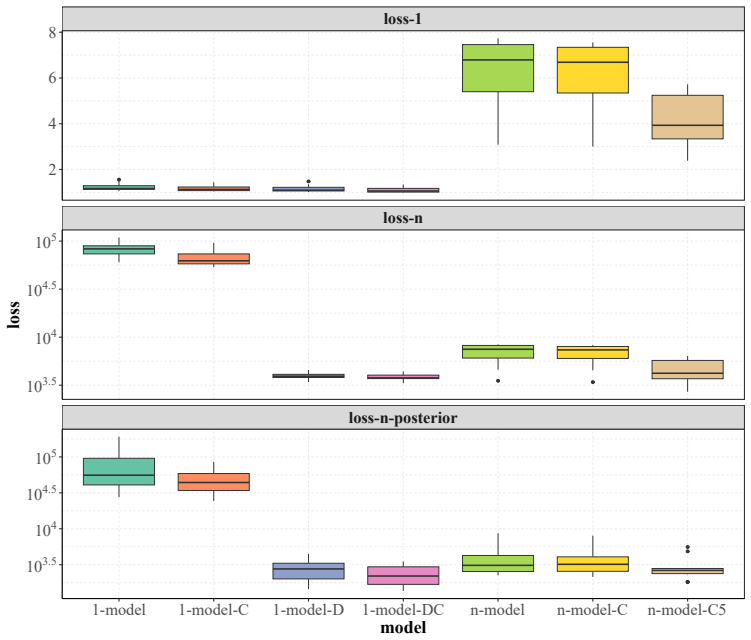
D” indicates debiasing and “C
Projection: min ψ Eq(θ) hψ(θ) − Epθs bϕ(θ, X) 2 When this procedure converges, we will get a score model within the mean-zero model family that minimizes the curvature regularized score loss. We find Algorithm 3 and the two alternatives have similar empirical performance in ou...
2019
Reviewed August 5, 2026 · model on record in the stance chip above.
Discussion (0). Continue with ORCID to comment.