REVIEW 4 major objections 4 minor 80 references
Plug-and-Play Latent Diffusion for Electromagnetic Inverse Scattering with Application to Brain Imaging
T0 review · 4 major / 4 minor · reviewed 2026-08-15 · deepseek-v4-flash
Pith's one-line read A latent-space plug-and-play diffusion sampler achieves state-of-the-art quantitative electromagnetic brain imaging without paired training data.
desk verdict Solid empirical paper on latent-space DPnP for EM inverse scattering; the theoretical guarantee is inherited rather than proven, and the UQ is thinner than claimed, but the reconstruction results deserve a serious referee. read the letter →
The pith
A machine-rendered reading of the paper's core claim, the machinery that carries it, and where it could break.
The reading
What carries the argument
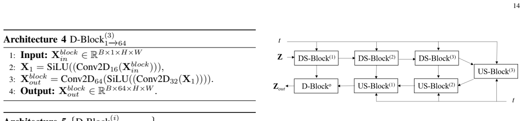
The load-bearing object is the learned latent space: a VAE encoder $E$ maps paired permittivity $\epsilon_r$ and conductivity $\sigma_e$ maps to a low-dimensional latent map $z$, and a decoder $G$ maps the latent back to physical maps. The Bayesian posterior is re-expressed as $p(z|d_{\mathrm{obs}}) \propto p(d_{\mathrm{obs}}|z)\,p(z)$, where the likelihood uses the composed nonlinear forward model $F(G(z))$ and $p(z)$ is captured by a score-based latent diffusion model. Sampling alternates a likelihood step, which draws from a proximal distribution $q_0(z|\hat{z}^k;\eta_k)$ via a Langevin SDE discretized with an exponential integrator, and a prior step, which draws from $q_1(z|\hat{z}^{k+1/2};\eta_k)$ by running the reverse-time diffusion SDE as a denoiser. The MMSE estimate is the average of $M$ decoded latent samples.
What would settle it
Run L-DPnP on synthetic brains with known ground truth, and compare its posterior samples with an exact reference posterior computed by a slower Markov-chain sampler on a small problem where that is feasible. If the L-DPnP sample mean is biased relative to the reference, or if its 90% credible intervals cover the true map in well under 90% of test cases, then the latent-space adaptation of the proximal-sampling guarantee is not holding and the reported RMSE advantage would not reflect true posterior sampling.
Extended reading notes
Core claim
L-DPnP replaces pixel-domain diffusion plug-and-play sampling with sampling in the latent space of a trained autoencoder, and claims that this change makes posterior sampling practical for nonlinear electromagnetic inverse scattering. On a 200-case ATLAS brain-imaging test the paper reports reconstruction RMSE of 0.075 and SSIM of 0.922, the best among the seven compared methods, while measurement RMSE of 0.192 stays close to the 20% noise level, indicating reconstructions that are both accurate and physically consistent. The same ranking pattern holds on MNIST and Fashion-MNIST-derived benchmarks. The paper attributes the improvement to a learned, material-aware latent representation that balances measurement sensitivities across latent coordinates, and to MMSE estimation over posterior samples rather than a single MAP reconstruction.
Load-bearing premise
Everything rests on the assumption that the alternating proximal sampler still converges to the true posterior $p(z|d_{\mathrm{obs}})$ when the prior step is a latent diffusion model inside a nonlinear autoencoder decoder; the paper provides no error bound for that adaptation.
Editorial extensions
If this is right
- On the ATLAS brain dataset, L-DPnP reports the lowest reconstruction RMSE (0.075) and highest SSIM (0.922) among the seven compared methods, with measurement RMSE (0.192) near the 20% noise level.
- Because the prior is learned from unlabeled property maps rather than from measurement-label pairs, the same trained prior can be reused when the antenna configuration or operating frequency changes.
- The sampler outputs multiple posterior draws, so the reconstruction comes with a per-pixel standard deviation map that flags unreliable regions.
- Working in the latent space balances the sensitivity of the unknown parameters to the measurements, cutting the number of alternating iterations from a practically infeasible value (about 200, ~6 hours) to 20 (~25 minutes) in the reported setup.
- MMSE averaging over samples avoids the overconfident single-map solutions that MAP-based methods such as GMR can produce.
Reading between the lines
- Beyond the paper, the latent-space sensitivity-balancing argument should transfer to other nonlinear inverse problems whose forward sensitivity varies across the domain, such as ultrasound tomography or electrical impedance tomography; the paper names these as future applications but does not test them.
- Beyond the paper, a controlled ablation that fixes the diffusion prior and varies only the autoencoder's latent dimension could separate how much of the reported gain comes from balanced gradients versus how much comes from the expressiveness of the learned prior.
- Beyond the paper, the claim that MMSE averaging avoids overconfident MAP solutions could be tested statistically on synthetic brains by comparing L-DPnP's posterior mean with single MAP draws across many cases, and by checking whether per-pixel variance tracks actual reconstruction error.
- Beyond the paper, since the convergence guarantee in [47] and [48] is proven for the pixel-domain setting, a natural falsifiable check is to compare L-DPnP samples on a small EM problem against brute-force MCMC to test posterior calibration.
Signed reviews
Editorial analysis
A structured set of objections, weighed in public.
Referee Report
Summary. The manuscript introduces L-DPnP, a latent-space plug-and-play posterior sampling algorithm for electromagnetic inverse scattering. A variational autoencoder is trained on unlabeled pairs of permittivity and conductivity maps, a score-based latent diffusion model is trained on the encoded latents, and at inference each posterior sample is produced by alternating a likelihood step (a Langevin/exponential-integrator update through the composed forward model F∘G) with a diffusion-based prior step; M decoded samples are averaged to approximate the MMSE estimate. The method is evaluated on MNIST, Fashion-MNIST, and ATLAS brain phantoms, where it reports the best reconstruction RMSE and SSIM among seven methods while keeping measurement RMSE near the noise level, and uncertainty maps are shown.
Significance. If the results hold, the paper describes a practically useful framework: it is, to my knowledge, the first application of latent-space diffusion posterior sampling to nonlinear electromagnetic inverse scattering, it avoids paired measurement-label training for the prior, and it is modular with respect to measurement geometry. The experimental comparison is solid in that all seven methods use the same forward model and the same test set, 200 cases per dataset, and the quantitative gains on ATLAS are substantial (reconstruction RMSE 0.075 versus 0.086 for the second-best method). The paper also provides detailed pseudocode and architecture descriptions. The main weakness is that the theoretical guarantee underlying the 'posterior sampling' framing is asserted rather than verified, and the implemented likelihood step contains a sign inconsistency and a heuristic adaptive rescaling; these issues do not disprove the empirical numbers, but they do undermine the theoretical claims as currently stated.
major comments (4)
- [Section IV-A, Eqs. (23)-(24)] The SDE written in (23) has dzτ = −∇L dτ + (1/η_k^2)(zτ−ż_k)dτ + √2 dwτ, but the exponential integrator (24) with r=e^{−γ/η^2} is the exact discretization of dzτ = +∇L dτ − (1/η_k^2)(zτ−ż_k)dτ + √2 dwτ. The signs of both the gradient term and the linear drift are opposite. Since Algorithm 2 and the implementation in Appendix B use (24), the derivation of the likelihood step as sampling q0 in (17) is internally inconsistent. The correct SDE for q0 is the one with the plus sign on ∇L and the minus sign on the linear drift, so the text should be corrected; as written, a reader cannot reproduce the algorithm from the equations.
- [Section III-C and Section VI-A] The convergence guarantee is imported from [47] and [48] without checking its hypotheses in the present setting. The likelihood here is the nonlinear composed map F∘G, where F includes the matrix inverse (I−G_D χ)^{−1} of (4), and the prior step is implemented by a learned score model rather than by the exact proximal distribution q1. Neither the regularity conditions of [48] (for example, Lipschitz or bounded-gradient assumptions, or linear-Gaussian structure) nor an error bound for the score approximation is stated. Moreover, the finite annealing schedule (η_k decreases only to 0.03 for ATLAS, with N_k=20 and M=5) is far from the asymptotic regime η→0, N_k→∞ used in the cited theory. Therefore the samples are not demonstrated to come from p(z|d_obs), and the MMSE estimate (12) and the uncertainty maps in Fig. 8 inherit this gap. This should be fixed either by proving the relevant conditions or by explicitly presenting the method as a heuristic sampler whose posterior accuracy is validated empirically.
- [Appendix B7, Eqs. (36)-(37)] The adaptive coefficient α_n in (37) multiplies the gradient term by a state-dependent factor proportional to ||z[n]||^2 / (||∇L(z[n])||^2 + 0.001). This rescaling is not the gradient of a fixed potential, and it changes the invariant measure of the likelihood-step chain; the choice of α_0 and the per-dataset η_k annealing schedules is hand-tuned. Consequently, even after the sign in (23) is corrected, the implemented likelihood step does not sample the proximal distribution q0 in (17). The paper should either justify this update as a valid MCMC kernel (for example, a preconditioned Langevin update with a known stationary distribution) or present it as a heuristic acceleration whose effect on the posterior is empirically assessed.
- [Section V-C and Fig. 8] Because the posterior-sampling guarantee is not established, and because the uncertainty maps are shown only for a few examples, the claim of 'reliable reconstruction' through MMSE and uncertainty quantification is under-supported. I would like to see a posterior predictive check, such as the coverage of credible intervals over the 200 test cases or a comparison between sample variance and actual reconstruction error, to demonstrate that the sample spread has calibration meaning despite the heuristic adaptations. Without such validation, Fig. 8 is an illustration rather than evidence of calibrated uncertainty.
minor comments (4)
- [Appendix B7, Eq. (36)] The second term on the right-hand side reads 'r x[n]' but should be 'r z[n]' to match the latent-space notation used elsewhere.
- [Algorithm 2, lines 11 and 20] The symbol n is used both as the discrete-time index and as the Gaussian noise vector; renaming one of them (for example, using ε for the noise realizations) would remove ambiguity.
- [Section II-A and Eq. (15)] The likelihood variance σ^2 in (15)-(16) is never specified in the experimental section; please state how it is set relative to the noise level in (31), since this parameter directly controls the strength of the likelihood step.
- [Table I and Section V-C] The paper reports that L-DPnP keeps measurement RMSE 'near the noise level'; because the noise in (31) is defined separately for the real and imaginary parts, a brief explanation of how the ATLAS value 0.192 compares with the 20% noise level would help interpret the table.
Circularity Check
No significant circularity: the derivation chain is self-contained, and the reported improvements are empirical posterior-sample estimates rather than fitted reconstructions.
full rationale
The central derivation is not circular. The prior p(z) is learned from unlabeled property maps, the likelihood (15)-(16) is built from the physical forward model F composed with the decoder G, and the MMSE estimate (12) is the sample average of decoded latent posterior samples. Nowhere are the reported reconstruction RMSE/SSIM values used as fit targets or normalization constants, so the quantitative claims are not forced by construction. The self-citations that appear, such as [41] for the VAE-style latent representation and [50] for the preliminary conference version, supply architecture choices, tissue property values, and prior context, but they do not carry the load of the posterior-sampling derivation or the SOTA claim. The convergence guarantee is imported from external works [47], [48], [49], not from the authors' own prior papers, and even though the transfer of that guarantee to the nonlinear latent forward model F∘G is asserted rather than verified (and the sign mismatch between SDE (23) and the discretized update (24) is an internal inconsistency), that is a rigorous-support gap rather than circularity, because the guarantee is not defined in terms of the outputs it claims to explain. The prior is trained on the same class of targets used for testing, which is standard Bayesian methodology and not a self-definitional reduction. Finally, the latent-space sensitivity argument in Section VI-A is an empirical explanation of faster convergence, not a redefinition of the reconstruction metric. Overall, no load-bearing step reduces to its own inputs.
Assumptions & free parameters
free parameters (3)
- alpha_0 gradient weighting =
0.3 (MNIST/Fashion-MNIST), 1 (ATLAS)
- eta_k annealing schedule =
0.4 to 0.1 (MNIST/Fashion-MNIST), 1 to 0.03 (ATLAS)
- Measurement noise variance sigma^2 =
Not explicitly stated
assumptions (4)
- domain assumption The alternating proximal sampling chain from Bouman and Buzzard [47] and Xu and Chi [48] converges to the posterior as eta -> 0.
- domain assumption The decoder G reconstructs (epsilon_r, sigma_e) with sufficient fidelity that F_G(z) = F(G(z)) is an accurate forward model.
- domain assumption The latent space gradients are balanced enough that the likelihood step updates all latent variables at similar rates.
- standard math The diffusion score model S approximates the true score of the latent prior after denoising score matching.
Cite this review
Pith. "Pith review of Plug-and-Play Latent Diffusion for Electromagnetic Inverse Scattering with Application to Brain Imaging." pith.science (2026). https://pith.science/paper/XW2FZIBE
@misc{pith2026250904860,
  author       = {Pith},
  title        = {Pith review of: Plug-and-Play Latent Diffusion for Electromagnetic Inverse Scattering with Application to Brain Imaging},
  year         = {2026},
  howpublished = {\url{https://pith.science/paper/XW2FZIBE}},
  note         = {Machine review of arXiv:2509.04860}
}
read the original abstract
Electromagnetic (EM) imaging is an important tool for non-invasive sensing with low-cost and portable devices. One emerging application is EM stroke imaging, which enables early diagnosis and continuous monitoring of brain strokes. Quantitative imaging is achieved by solving an inverse scattering problem (ISP) that reconstructs permittivity and conductivity maps from measurements. In general, the reconstruction accuracy is limited by its inherent nonlinearity and ill-posedness. Existing methods, including learning-free and learning-based approaches, fail to either incorporate complicated prior distributions or provide theoretical guarantees, posing difficulties in balancing interpretability, distortion error, and reliability. To overcome these limitations, we propose a posterior sampling method based on latent diffusion for quantitative EM brain imaging, adapted from a generative plug-and-play (PnP) posterior sampling framework. Our approach allows to flexibly integrate prior knowledge into physics-based inversion without requiring paired measurement-label datasets. We first learn the prior distribution of targets from an unlabeled dataset, and then incorporate the learned prior into posterior sampling. In particular, we train a latent diffusion model on permittivity and conductivity maps to capture their prior distribution. Then, given measurements and the forward model describing EM wave physics, we perform posterior sampling by alternating between two samplers that respectively enforce the likelihood and prior distributions. Finally, reliable reconstruction is obtained through minimum mean squared error (MMSE) estimation based on the samples. Experimental results on brain imaging demonstrate that our approach achieves state-of-the-art performance in reconstruction accuracy and structural similarity while maintaining high measurement fidelity.
Figures


Figures from the paper (8 more)


Reference graph
Works this paper leans on
-
[47]
Generative plug and play: Posterior sampling for inverse problems,
C. A. Bouman and G. T. Buzzard, “Generative plug and play: Posterior sampling for inverse problems,” in2023 59th Annual Allerton Confer- ence on Communication, Control, and Computing (Allerton), pp. 1–7, 2023
work page 2023
-
[48]
Provably robust score-based diffusion posterior sampling for plug-and-play image reconstruction,
X. Xu and Y . Chi, “Provably robust score-based diffusion posterior sampling for plug-and-play image reconstruction,”Advances in Neural Information Processing Systems, 2024. 18
work page 2024
- [1]
- [2]
-
[3]
K. Tan, X. Chen, S. Wu, and G. Fang, “Efficient frequency scaling algorithm for short-range 3-D holographic imaging based on a scanning MIMO array,”IEEE Transactions on Microwave Theory and Techniques, vol. 68, no. 9, pp. 3885–3897, 2020. 17
work page 2020
-
[4]
X. Zhang and X. Ye, “Solving strongly nonlinear inverse scattering prob- lems for mixture of dielectric and PEC with novel contraction T-matrix equation,”IEEE Transactions on Microwave Theory and Techniques, 2025
work page 2025
-
[5]
Instantaneous brain stroke classification and localization from real scattering data,
M. Salucci, A. Gelmini, J. Vrba, I. Merunka, G. Oliveri, and P. Rocca, “Instantaneous brain stroke classification and localization from real scattering data,”Microwave and Optical Technology Letters, vol. 61, no. 3, pp. 805–808, 2019
work page 2019
-
[6]
Millimeter-waves breast cancer imaging via inverse scattering tech- niques,
M. T. Bevacqua, S. Di Meo, L. Crocco, T. Isernia, and M. Pasian, “Millimeter-waves breast cancer imaging via inverse scattering tech- niques,”IEEE Journal of Electromagnetics, RF and Microwaves in Medicine and Biology, 2021
work page 2021
Show all 80 references
-
[7]
A physics-driven AI approach for microwave imaging of breast tumors,
F. Zardi, L. Tosi, M. Salucci, and A. Massa, “A physics-driven AI approach for microwave imaging of breast tumors,”IEEE Transactions on Antennas and Propagation, 2025
2025
-
[8]
A microwave imaging method for NDE/NDT based on the SMW technique for the electromagnetic field prediction,
A. Massa, M. Pastorino, A. Rosani, and M. Benedetti, “A microwave imaging method for NDE/NDT based on the SMW technique for the electromagnetic field prediction,”IEEE Transactions on Instrumentation and Measurement, vol. 55, no. 1, pp. 240–247, 2006
2006
-
[9]
Zoughi,Microwave non-destructive testing and evaluation principles, vol
R. Zoughi,Microwave non-destructive testing and evaluation principles, vol. 4. Springer Science & Business Media, 2000
2000
-
[10]
Electromagnetic tomography for brain imaging and stroke diagnostics: Progress towards clinical application,
A. Hamidipour, T. Henriksson, M. Hopfer, R. Planas, and S. Semenov, “Electromagnetic tomography for brain imaging and stroke diagnostics: Progress towards clinical application,” inEmerging electromagnetic technologies for brain diseases diagnostics, monitoring and therapy, pp....
2018
-
[11]
A review of current imaging methods used in stroke research,
H.-Y . Wey, V . R. Desai, and T. Q. Duong, “A review of current imaging methods used in stroke research,”Neurological research, vol. 35, no. 10, pp. 1092–1102, 2013
2013
-
[12]
Chen,Computational methods for electromagnetic inverse scattering
X. Chen,Computational methods for electromagnetic inverse scattering. John Wiley & Sons, 2018
2018
-
[13]
On the degrees of freedom of scattered fields,
O. M. Bucci and G. Franceschetti, “On the degrees of freedom of scattered fields,”IEEE transactions on Antennas and Propagation, vol. 37, no. 7, pp. 918–926, 1989
1989
-
[14]
Application of the multiplicative regularized Gauss–Newton algorithm for three- dimensional microwave imaging,
A. Abubakar, T. M. Habashy, G. Pan, and M.-K. Li, “Application of the multiplicative regularized Gauss–Newton algorithm for three- dimensional microwave imaging,”IEEE Transactions on Antennas and Propagation, vol. 60, no. 5, pp. 2431–2441, 2012
2012
-
[15]
Imaging of biomedical data using a multiplicative regularized contrast source inversion method,
A. Abubakar, P. van den Berg, and J. Mallorqui, “Imaging of biomedical data using a multiplicative regularized contrast source inversion method,” IEEE Transactions on Microwave Theory and Techniques, vol. 50, no. 7, pp. 1761–1771, 2002
2002
-
[16]
Alternating direction method of multiplier for solving electromagnetic inverse scattering problems,
J. Liu, H. Zhou, L. Chen, and T. Ouyang, “Alternating direction method of multiplier for solving electromagnetic inverse scattering problems,” International Journal of Microwave and Wireless Technologies, vol. 12, no. 8, pp. 790–796, 2020
2020
-
[17]
Bayesian inversion and sampling methods,
Q. Shen, J. Chen, X. Wu, Y . Huang, Z. Han, Q. Shen, J. Chen, X. Wu, Y . Huang, and Z. Han, “Bayesian inversion and sampling methods,” Statistical Inversion of Electromagnetic Logging Data, pp. 17–29, 2021
2021
-
[18]
3-D bayesian variational full waveform inversion,
X. Zhang, A. Lomas, M. Zhou, Y . Zheng, and A. Curtis, “3-D bayesian variational full waveform inversion,”Geophysical Journal International, vol. 234, no. 1, pp. 546–561, 2023
2023
-
[19]
Bayesian inversion of frequency-domain airborne em data with spatial correlation prior information,
J. Zhou, D. Husmeier, H. Gao, C. Yin, C. Qiu, X. Jing, Y . Qi, and W. Liu, “Bayesian inversion of frequency-domain airborne em data with spatial correlation prior information,”IEEE Transactions on Geoscience and Remote Sensing, vol. 62, pp. 1–16, 2024
2024
-
[20]
A three-dimensional model- based inversion algorithm using radial basis functions for microwave data,
M. Li, A. Abubakar, and T. M. Habashy, “A three-dimensional model- based inversion algorithm using radial basis functions for microwave data,”IEEE Transactions on Antennas and Propagation, vol. 60, no. 7, pp. 3361–3372, 2012
2012
-
[21]
Microwave imaging of nonsparse domains using Born iterative method with wavelet transform and block sparse Bayesian learning,
L. Guo and A. M. Abbosh, “Microwave imaging of nonsparse domains using Born iterative method with wavelet transform and block sparse Bayesian learning,”IEEE Transactions on Antennas and Propagation, vol. 63, no. 11, pp. 4877–4888, 2015
2015
-
[22]
A review of deep learning approaches for inverse scattering problems (invited review),
X. Chen, Z. Wei, L. Maokun, P. Rocca,et al., “A review of deep learning approaches for inverse scattering problems (invited review),” Electromagnetic Waves, vol. 167, pp. 67–81, 2020
2020
-
[23]
DeepNIS: Deep neural network for nonlinear electromagnetic inverse scattering,
L. Li, L. G. Wang, F. L. Teixeira, C. Liu, A. Nehorai, and T. J. Cui, “DeepNIS: Deep neural network for nonlinear electromagnetic inverse scattering,”IEEE Transactions on Antennas and Propagation, vol. 67, no. 3, pp. 1819–1825, 2018
2018
-
[24]
Machine learning in electromagnetics with applications to biomedical imaging: A review,
M. Li, R. Guo, K. Zhang, Z. Lin, F. Yang, S. Xu, X. Chen, A. Massa, and A. Abubakar, “Machine learning in electromagnetics with applications to biomedical imaging: A review,”IEEE Antennas and Propagation Magazine, vol. 63, no. 3, pp. 39–51, 2021
2021
-
[25]
J. C. Ye, Y . C. Eldar, and M. Unser,Deep Learning for Biomedical Image Reconstruction. Cambridge University Press, 2023
2023
-
[26]
Physics-embedded machine learning for electromagnetic data imaging: Examining three types of data-driven imaging methods,
R. Guo, T. Huang, M. Li, H. Zhang, and Y . C. Eldar, “Physics-embedded machine learning for electromagnetic data imaging: Examining three types of data-driven imaging methods,”IEEE Signal Processing Maga- zine, vol. 40, no. 2, pp. 18–31, 2023
2023
-
[27]
Free space experimental scattering database continuation: experimental set-up and measurement precision,
J.-M. Geffrin, P. Sabouroux, and C. Eyraud, “Free space experimental scattering database continuation: experimental set-up and measurement precision,”Inverse Problems, vol. 21, no. 6, p. S117, 2005
2005
-
[28]
Algorithm unrolling: Interpretable, efficient deep learning for signal and image processing,
V . Monga, Y . Li, and Y . C. Eldar, “Algorithm unrolling: Interpretable, efficient deep learning for signal and image processing,”IEEE Signal Processing Magazine, vol. 38, no. 2, pp. 18–44, 2021
2021
-
[29]
Model-based deep learning: On the intersection of deep learning and optimization,
N. Shlezinger, Y . C. Eldar, and S. P. Boyd, “Model-based deep learning: On the intersection of deep learning and optimization,”IEEE Access, vol. 10, pp. 115384–115398, 2022
2022
-
[30]
Deep-learning schemes for full-wave nonlinear inverse scattering problems,
Z. Wei and X. Chen, “Deep-learning schemes for full-wave nonlinear inverse scattering problems,”IEEE Transactions on Geoscience and Remote Sensing, vol. 57, no. 4, pp. 1849–1860, 2018
2018
-
[31]
An inhomogeneous background imaging method based on generative adversarial network,
X. Ye, Y . Bai, R. Song, K. Xu, and J. An, “An inhomogeneous background imaging method based on generative adversarial network,” IEEE Transactions on Microwave Theory and Techniques, vol. 68, no. 11, pp. 4684–4693, 2020
2020
-
[32]
Deep unfolding of full waveform inversion for quantitative ultrasound imaging,
N. Cohen, Y . Kvich, R. Guo, and Y . C. Eldar, “Deep unfolding of full waveform inversion for quantitative ultrasound imaging,” inICASSP 2025-2025 IEEE International Conference on Acoustics, Speech and Signal Processing (ICASSP), pp. 1–5, IEEE, 2025
2025
-
[33]
A physics-driven deep- learning network for solving nonlinear inverse problems,
Y . Jin, Q. Shen, X. Wu, J. Chen, and Y . Huang, “A physics-driven deep- learning network for solving nonlinear inverse problems,”Petrophysics, vol. 61, no. 01, pp. 86–98, 2020
2020
-
[34]
Strong solutions for PDE-based tomography by unsupervised learning,
L. Bar and N. Sochen, “Strong solutions for PDE-based tomography by unsupervised learning,”SIAM Journal on Imaging Sciences, vol. 14, no. 1, pp. 128–155, 2021
2021
-
[35]
Real-time model-based quantitative ultra- sound and radar,
T. Sharon and Y . C. Eldar, “Real-time model-based quantitative ultra- sound and radar,”IEEE Transactions on Computational Imaging, vol. 10, pp. 1175–1190, 2024
2024
-
[36]
Physics embedded deep neural network for solving full- wave inverse scattering problems,
R. Guo, Z. Lin, T. Shan, X. Song, M. Li, F. Yang, S. Xu, and A. Abubakar, “Physics embedded deep neural network for solving full- wave inverse scattering problems,”IEEE Transactions on Antennas and Propagation, vol. 70, no. 8, pp. 6148–6159, 2021
2021
-
[37]
Plug-and-play priors for model based reconstruction,
S. V . Venkatakrishnan, C. A. Bouman, and B. Wohlberg, “Plug-and-play priors for model based reconstruction,” in2013 IEEE Global Conference on Signal and Information Processing, pp. 945–948, IEEE, 2013
2013
-
[38]
Compressed sensing using generative models,
A. Bora, A. Jalal, E. Price, and A. G. Dimakis, “Compressed sensing using generative models,” inInternational Conference on Machine Learning, pp. 537–546, PMLR, 2017
2017
-
[39]
Deep image prior,
D. Ulyanov, A. Vedaldi, and V . Lempitsky, “Deep image prior,” in Proceedings of the IEEE Conference on Computer Vision and Pattern Recognition, pp. 9446–9454, 2018
2018
-
[40]
DeepEIT: Deep image prior enabled electrical impedance tomography,
D. Liu, J. Wang, Q. Shan, D. Smyl, J. Deng, and J. Du, “DeepEIT: Deep image prior enabled electrical impedance tomography,”IEEE Transactions on Pattern Analysis and Machine Intelligence, vol. 45, no. 8, pp. 9627–9638, 2023
2023
-
[41]
Three dimensional microwave data inversion in feature space for stroke imaging,
R. Guo, Z. Lin, J. Xin, M. Li, F. Yang, S. Xu, and A. Abubakar, “Three dimensional microwave data inversion in feature space for stroke imaging,”IEEE Transactions on Medical Imaging, vol. 43, no. 4, pp. 1365–1376, 2024
2024
-
[42]
Deep injective prior for inverse scattering,
A. Khorashadizadeh, V . Khorashadizadeh, S. Eskandari, G. A. E. Van- denbosch, and I. Dokmani´c, “Deep injective prior for inverse scattering,” IEEE Transactions on Antennas and Propagation, vol. 71, no. 11, pp. 8894–8906, 2023
2023
-
[43]
Stochastic solutions for linear inverse problems using the prior implicit in a denoiser,
Z. Kadkhodaie and E. Simoncelli, “Stochastic solutions for linear inverse problems using the prior implicit in a denoiser,”Advances in Neural Information Processing Systems, vol. 34, pp. 13242–13254, 2021
2021
-
[44]
Diffusion posterior sampling for general noisy inverse problems,
H. Chung, J. Kim, M. T. Mccann, M. L. Klasky, and J. C. Ye, “Diffusion posterior sampling for general noisy inverse problems,” inThe Eleventh International Conference on Learning Representations, 2023
2023
-
[45]
Denoising diffusion restoration models,
B. Kawar, M. Elad, S. Ermon, and J. Song, “Denoising diffusion restoration models,”Advances in Neural Information Processing Sys- tems, vol. 35, pp. 23593–23606, 2022
2022
-
[46]
Solving inverse problems in medical imaging with score-based generative models,
Y . Song, L. Shen, L. Xing, and S. Ermon, “Solving inverse problems in medical imaging with score-based generative models,” inInternational Conference on Learning Representations, 2022
2022
-
[49]
Prin- cipled probabilistic imaging using diffusion models as plug-and-play priors,
Z. Wu, Y . Sun, Y . Chen, B. Zhang, Y . Yue, and K. Bouman, “Prin- cipled probabilistic imaging using diffusion models as plug-and-play priors,”Advances in Neural Information Processing Systems, vol. 37, pp. 118389–118427, 2024
2024
-
[50]
Posterior sampling with latent diffusion for microwave brain imaging,
R. Guo, Y . Kvich, Y . Zhang, T. Huang, M. Li, and C. Y . Eldar, “Posterior sampling with latent diffusion for microwave brain imaging,” in47th Annual International Conference of the IEEE Engineering in Medicine and Biology Society, p. to be appeared, 2025
2025
-
[51]
Jin,Theory and computation of electromagnetic fields
J.-M. Jin,Theory and computation of electromagnetic fields. John Wiley & Sons, 2015
2015
-
[52]
The metropo- lis—hastings algorithm,
C. P. Robert, G. Casella, C. P. Robert, and G. Casella, “The metropo- lis—hastings algorithm,”Monte Carlo statistical methods, pp. 267–320, 2004
2004
-
[53]
Optimal scaling of discrete approxi- mations to Langevin diffusions,
G. O. Roberts and J. S. Rosenthal, “Optimal scaling of discrete approxi- mations to Langevin diffusions,”Journal of the Royal Statistical Society: Series B (Statistical Methodology), vol. 60, no. 1, pp. 255–268, 1998
1998
-
[54]
Score-based generative modeling through stochastic differ- ential equations,
Y . Song, J. Sohl-Dickstein, D. P. Kingma, A. Kumar, S. Ermon, and B. Poole, “Score-based generative modeling through stochastic differ- ential equations,” inInternational Conference on Learning Representa- tions, 2021
2021
-
[55]
Denoising diffusion probabilistic models,
J. Ho, A. Jain, and P. Abbeel, “Denoising diffusion probabilistic models,” Advances in Neural Information Processing Systems, vol. 33, pp. 6840– 6851, 2020
2020
-
[56]
Diffusion models in low-level vision: A survey,
C. He, Y . Shen, C. Fang, F. Xiao, L. Tang, Y . Zhang, W. Zuo, Z. Guo, and X. Li, “Diffusion models in low-level vision: A survey,”IEEE Transactions on Pattern Analysis and Machine Intelligence, 2025
2025
-
[57]
Diffusion models, image super-resolution, and everything: A survey,
B. B. Moser, A. S. Shanbhag, F. Raue, S. Frolov, S. Palacio, and A. Dengel, “Diffusion models, image super-resolution, and everything: A survey,”IEEE Transactions on Neural Networks and Learning Systems, 2024
2024
-
[58]
S ¨arkk¨a and A
S. S ¨arkk¨a and A. Solin,Applied stochastic differential equations, vol. 10. Cambridge University Press, 2019
2019
-
[59]
A connection between score matching and denoising au- toencoders,
P. Vincent, “A connection between score matching and denoising au- toencoders,”Neural Computation, vol. 23, no. 7, pp. 1661–1674, 2011
2011
-
[60]
P. E. Kloeden, E. Platen, P. E. Kloeden, and E. Platen,Stochastic differential equations. Springer, 1992
1992
-
[61]
Gradient-based learning applied to document recognition,
Y . Lecun, L. Bottou, Y . Bengio, and P. Haffner, “Gradient-based learning applied to document recognition,”Proceedings of the IEEE, vol. 86, no. 11, pp. 2278–2324, 1998
1998
-
[62]
Fashion-MNIST: a novel image dataset for benchmarking machine learning algorithms,
H. Xiao, K. Rasul, and R. V ollgraf, “Fashion-MNIST: a novel image dataset for benchmarking machine learning algorithms,”arXiv preprint arXiv:1708.07747, 2017
2017 arXiv
-
[63]
A large, open source dataset of stroke anatomical brain images and manual lesion segmentations,
S.-L. Liew, J. M. Anglin, N. W. Banks, M. Sondag, K. L. Ito, H. Kim, J. Chan, J. Ito, C. Jung, N. Khoshab,et al., “A large, open source dataset of stroke anatomical brain images and manual lesion segmentations,” Scientific Data, vol. 5, no. 1, pp. 1–11, 2018
2018
-
[64]
Occam’s inversion: A practical algorithm for generating smooth models from electromag- netic sounding data,
S. C. Constable, R. L. Parker, and C. G. Constable, “Occam’s inversion: A practical algorithm for generating smooth models from electromag- netic sounding data,”Geophysics, vol. 52, no. 3, pp. 289–300, 1987
1987
-
[65]
ADMM-based multipa- rameter wavefield reconstruction inversion in VTI acoustic media with TV regularization,
H. S. Aghamiry, A. Gholami, and S. Operto, “ADMM-based multipa- rameter wavefield reconstruction inversion in VTI acoustic media with TV regularization,”Geophysical Journal International, vol. 219, no. 2, pp. 1316–1333, 2019
2019
-
[66]
DeepNIS: Deep neural network for nonlinear electromagnetic inverse scattering,
L. Li, L. G. Wang, F. L. Teixeira, C. Liu, A. Nehorai, and T. J. Cui, “DeepNIS: Deep neural network for nonlinear electromagnetic inverse scattering,”IEEE Transactions on Antennas and Propagation, vol. 67, no. 3, pp. 1819–1825, 2019
2019
-
[67]
High- resolution image synthesis with latent diffusion models,
R. Rombach, A. Blattmann, D. Lorenz, P. Esser, and B. Ommer, “High- resolution image synthesis with latent diffusion models,” inProceedings of the IEEE/CVF conference on computer vision and pattern recognition, pp. 10684–10695, 2022
2022
-
[68]
Denoising diffusion implicit models,
J. Song, C. Meng, and S. Ermon, “Denoising diffusion implicit models,” arXiv preprint arXiv:2010.02502, 2020
2010 arXiv
-
[69]
DPM-solver: A fast ODE solver for diffusion probabilistic model sampling in around 10 steps,
C. Lu, Y . Zhou, F. Bao, J. Chen, C. Li, and J. Zhu, “DPM-solver: A fast ODE solver for diffusion probabilistic model sampling in around 10 steps,”Advances in Neural Information Processing Systems, vol. 35, pp. 5775–5787, 2022
2022
-
[70]
Three-dimensional electrical impedance tomography with multiplicative regularization,
K. Zhang, M. Li, F. Yang, S. Xu, and A. Abubakar, “Three-dimensional electrical impedance tomography with multiplicative regularization,” IEEE Transactions on Biomedical Engineering, vol. 66, no. 9, pp. 2470– 2480, 2019
2019
-
[71]
Quantita- tive ultrasound brain imaging with multiscale deconvolutional waveform inversion,
Y .-B. Li, J. Wang, C. Su, W.-J. Lin, X.-M. Wang, and Y . Luo, “Quantita- tive ultrasound brain imaging with multiscale deconvolutional waveform inversion,”Chinese Physics B, vol. 32, no. 1, p. 014303, 2023
2023
-
[72]
Recent advances in machine learning-enhanced joint inversion of seismic and electromag- netic data,
J. Ma, Y . Deng, X. Li, R. Guo, H. Zhou, and M. Li, “Recent advances in machine learning-enhanced joint inversion of seismic and electromag- netic data,”Surveys in Geophysics, pp. 1–29, 2024
2024
-
[73]
Deep joint inversion of multiple geophysical data with U-net reparameterization,
R. Guo, H. Zhou, X. Wei, Z. Lin, M. Li, Y . C. Eldar, F. Yang, S. Xu, and A. Abubakar, “Deep joint inversion of multiple geophysical data with U-net reparameterization,”Geophysics, vol. 90, no. 3, pp. W A61–W A75, 2024
2024
-
[74]
Three-dimensional joint inversion of EM and acoustic data based on contrast source inversion,
X. Song, M. Li, F. Yang, S. Xu, and A. Abubakar, “Three-dimensional joint inversion of EM and acoustic data based on contrast source inversion,”IEEE Journal on Multiscale and Multiphysics Computational Techniques, vol. 5, pp. 28–36, 2020
2020
-
[75]
Auto-Encoding variational Bayes,
D. P. Kingma and M. Welling, “Auto-Encoding variational Bayes,” in 2nd International Conference on Learning Representations, ICLR 2014, Banff, AB, Canada, April 14-16, 2014, Conference Track Proceedings, 2014
2014
-
[76]
Generating diverse high-fidelity images with VQ-V AE-2,
A. Razavi, A. Van den Oord, and O. Vinyals, “Generating diverse high-fidelity images with VQ-V AE-2,”Advances in Neural Information Processing Systems, vol. 32, 2019
2019
-
[77]
Variational autoencoder for deep learning of images, labels and cap- tions,
Y . Pu, Z. Gan, R. Henao, X. Yuan, C. Li, A. Stevens, and L. Carin, “Variational autoencoder for deep learning of images, labels and cap- tions,”Advances in Neural Information Processing Systems, vol. 29, pp. 2352–2360, 2016
2016
-
[78]
On the limited memory BFGS method for large scale optimization,
D. C. Liu and J. Nocedal, “On the limited memory BFGS method for large scale optimization,”Mathematical Programming, vol. 45, no. 1, pp. 503–528, 1989
1989
-
[79]
Adam: A method for stochastic optimization,
D. P. Kingma and J. Ba, “Adam: A method for stochastic optimization,” arXiv preprint arXiv:1412.6980, 2014
2014 arXiv
-
[80]
Tutorial on variational autoencoders,
C. Doersch, “Tutorial on variational autoencoders,”arXiv preprint arXiv:1606.05908, 2016
2016 arXiv
Reviewed August 15, 2026 · model on record in the stance chip above.
Discussion (0). Continue with ORCID to comment.