Treatment Effects of Multi-Valued Treatments in Hyper-Rectangle Model

Xunkang Tian

REVIEW 4 major objections 3 minor 25 references

Treatment Effects of Multi-Valued Treatments in Hyper-Rectangle Model

T0 review · 4 major / 3 minor · reviewed 2026-08-05 · deepseek-v4-flash

Challenge this review Re-run · record.json Download PDF Read on arXiv ↗

Pith's one-line read Sharp identification of multi-valued treatment effects via ranked-treatment bounds.

desk verdict A mostly sound restatement of Lee-Salanie weighed down by a load-bearing copula identification that does not work, plus a faulty sharpness proof and an invalid policy test; send to referees, but the central new claims likely will not survive. read the letter →

arxiv 2509.05177 v1 pith:CET7NMW5 submitted 2025-09-05 econ.EM

Xunkang Tian This is my paper

classification econ.EM MSC 62P2062G05

keywords multi-valuedtreatmentmarginalresponsesetidentificationhyper-rectanglemodelpolicyrelevanteffectmonotoneinstrumentalvariablesleadingterm

verification ladder T0 review T1 audit T2 compute T3 formal

The pith

A machine-rendered reading of the paper's core claim, the machinery that carries it, and where it could break.

The reading

Drawing on the hyper-rectangle model of multi-valued treatment assignment, this paper asks when the marginal treatment response E[Y_k|V=v] can be recovered from data on instruments, thresholds, and outcomes. It shows that when a treatment's assignment rule involves all dimensions of unobserved heterogeneity (a full-rank 'leading term'), the MTR is point identified by differentiating observed moments. When no such full-rank term exists, adding a ranked-treatment assumption—higher treatment levels have weakly larger expected outcomes given V—yields sharp set identification. The paper also derives identified sets for ATE, ATT, LATE, and policy-relevant treatment effects, and provides hypothesis tests for policy effectiveness under point and partial identification. The practical payoff: researchers can bound treatment effects in multi-valued settings without knowing assignment thresholds or forcing treatment to depend on all unobserved heterogeneity.

What carries the argument

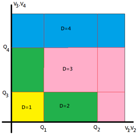
The leading-term decomposition d_k(V,Q(Z)) = Σ_{l∈L} c^k_l Π_{j∈l} S_j(V,Q(Z)). The leading terms are the inclusion-maximal monomials; their rank |l| is the number of unobserved-heterogeneity dimensions they touch. This object carries the argument because differentiation with respect to the corresponding threshold coordinates cancels all subterms, isolating either the joint density of V (Section 3) or a conditional MTR (Section 4). When no leading term has full rank, Assumption 9's ordering constraints—E[Y_{κ'}|V] ≤ E[Y_κ|V] for κ' < κ—supply the missing information that turns the conditional MTR equalities into bounds.

What would settle it

Simulate a two-dimensional model with known thresholds, no full-rank leading term, and V drawn from a copula with dependence parameter ρ. Compute the marginal distributions from Pr(D=k|Q(Z)=q), fit the copula by the paper's MLE procedure, and check whether the estimate of ρ converges to the true value. If it does not—because the likelihood is flat in ρ—then Section 4.2's conditional densities are misspecified and the nominal identified set can exclude the true E[Y_k|V=v].

Watch

Extended reading notes

Core claim

Treatment selection is modeled as a measurable function of threshold indicators S_j(V,Q(Z))=1{V_j<Q_j(Z)}. Each treatment's indicator is expanded as a signed sum of products of these indicators; a term is leading if no other term contains it. For a full-rank leading term, differentiating observed conditional moments E[Y D_k|Q(Z)=q] with respect to all q-coordinates isolates c E[Y_k|V=q] f_V(q), giving point identification of the MTR almost everywhere. Without a full-rank leading term, differentiation along a leading term's coordinates only identifies the conditional MTR E[Y_k|V_{I^+_l}=v], averaged over the other coordinates of V. The paper's central claim is that the ranked-treatment assump

Load-bearing premise

In the non-full-rank case, the paper assumes the joint distribution of the unobserved heterogeneity can be recovered by fitting a correctly specified copula to the marginal distributions identified from data; if that copula family is wrong or its dependence parameters are not identified, the conditional densities used in the Section 4.2 bounds and the sharpness claims do not follow.

Editorial extensions

If this is right

For any treatment level whose leading term is full rank, the marginal treatment response is point identified almost everywhere, extending the baseline hyper-rectangle results to settings where thresholds or the distribution of V may be unknown (one of them known).
For treatments lacking a full-rank leading term, the ranked-treatment assumption yields a sharp identified set for the MTR; all ATE, ATT, LATE, and policy-relevant treatment parameters that are linear functionals of MTRs inherit corresponding identified sets.
With known thresholds, the distribution of unobserved heterogeneity can be recovered even without full-rank leading terms provided a correctly specified copula family is available.
With known distribution of V, threshold functions are point identified when the rank condition J ≤ rank{c^k_l} holds, and can be approximated consistently by a parametric sieve.
The paper's policy test remains valid when MTRs are only set-identified, using a confidence interval that asymptotically covers the true policy effect with at least the nominal probability.

Reading between the lines

Editorial extensions of the paper, not claims the author makes directly.

A natural robustness check the paper does not report: since the non-full-rank case needs a copula family, the identified set should be re-computed over a range of copula families, because the reported bounds are conditional on the chosen family.
The ranked-treatment assumption is testable in data when at least one treatment has a full-rank leading term, since then the ordering of conditional means is point identified and can be compared against the assumption.
The policy-testing framework extends directly to one-sided questions (does the policy improve welfare?) by replacing the two-sided interval with one-sided confidence bounds.
Because the bounds tighten as leading terms cover more dimensions of V, instrument design could aim for thresholds that vary along multiple heterogeneity dimensions rather than one.

Share X Bluesky LinkedIn Reddit HN

Editorial analysis

A structured set of objections, weighed in public.

Desk editor's note, referee report, and a circularity audit.

Desk Editor's Note

read the letter

Colleague, this one is worth a look, but not for the reasons the abstract suggests. The sound part is the re-derivation of Lee-Salanié: the leading-term decomposition and the full-rank differentiation results are clean and correctly reproduced. If you need a self-contained account of that machinery, this preprint is actually a useful read. The new material, though, falls down exactly where it claims to extend the literature.

The set-identification route (Section 4.2) depends on the joint density f_V, which Section 3.1.2 claims to recover from leading-term marginals via a copula. That does not work. The paper applies Sklar's theorem to multivariate marginal CDFs F_{I^+_l}; Sklar is for univariate margins, so the representation is not even a valid copula. More importantly, even if one granted some multivariate Sklar, the copula parameters are not identified from the observed treatment probabilities — those probabilities identify only the marginals on the leading-term coordinates. Steps 4 and 5 of Section 3.1.2 generate a synthetic sample from the assumed copula and run MLE on it; that recovers the assumption, not the data. The conditional densities in (4.7)–(4.8) are therefore choice variables, and Theorems 4.1 and 4.2 do not describe the data-identified set.

There is a second issue in Lemma A.1's proof, where the boundary condition Ψ_k(q)=0 for any coordinate q_j=0 fails when treatment k's leading terms do not involve dimension j — Example 1's d1=S2S3 is a direct counterexample. That may be repairable by restricting to coordinates in the union of leading terms, but as stated it's false.

The policy test in Section 6 is also not a test about the true GPRTE: it treats Monte Carlo draws from a known distribution as the sampling variation, letting M→∞ with N0 fixed, and never accounts for estimation error in f_V or the MTRs. The Imbens–Manski coverage argument is invoked, but its premises are not met.

So: the Lee-Salanié core is fine, the claimed extensions are not. A serious referee could make these points quickly; the paper probably would not survive, even with revision, because the copula identification is load-bearing and unfixable within the current setup. Still, the topic matters and the writing is clear enough that it deserves to be read by someone working on multi-valued treatments — I'd send it to a referee rather than desk-reject it, so that the flaws are on record. I wouldn't cite it in its present form.

Referee Report

4 major / 3 minor

Summary. This paper extends the Lee-Salanié (2018) hyper-rectangle model of multi-valued treatment. Treatment D=k is determined by a polynomial in indicators {V_j<Q_j(Z)}, and the paper introduces 'leading terms' to organize the identification analysis. Section 3 studies identification of the threshold function Q(Z) when the distribution of V is known and of f_V when the thresholds are known. Section 4 identifies E[Y_k|V=v] by differentiation when a full-rank leading term exists, and proposes set identification under a monotone 'ranked treatment' assumption when no full-rank leading term exists. Sections 5-6 derive treatment effects and a policy-relevant hypothesis test. The full-rank differentiation parts are standard, but the new non-full-rank identification, the sharpness proofs, the unknown-threshold theorem, and the testing framework contain load-bearing gaps.

Significance. If the new results were correct, the paper would extend the Lee-Salanié framework to settings with unknown thresholds and to treatments whose leading terms are not full rank, and it would add a practical policy test. The full-rank derivative identification in Sections 3.1.1 and 4.1 is clean and essentially correct given the regularity assumptions, and the leading-term taxonomy is potentially useful. The idea of applying Manski-style monotone response to bound MTRs is also sensible. However, the central novel claim—set identification of E[Y_k|V] when no treatment has a full-rank leading term—depends on an unidentified copula model for the joint distribution of V. The sharpness arguments are incomplete, the unknown-threshold identification theorem rests on an insufficient rank argument, and the policy test ignores first-stage estimation error. Because the load-bearing new contributions are not established, the paper is not suitable for publication in its current form.

major comments (4)

[Section 3.1.2] The claimed identification of f_V absent a full-rank leading term is not valid. The equation after Sklar's theorem states F_V(v)=C(F_{I^+_l1}(v),...,F_{I^+_lP}(v);β_C). Sklar's theorem applies to univariate marginals; the arguments here are multivariate CDFs of blocks I^+_l, whose probability integral transforms are not Uniform(0,1). More importantly, data identify only the leading-term marginals in (3.2); the copula parameters are estimated in Steps 4-5 by generating a synthetic sample from the assumed copula and running MLE on that sample, so β̂_C recovers the assumed dependence, not information in the data. Hence f_V and the conditional densities f_{I^-|I^+} used in (4.7)-(4.8) are not identified, and Theorems 4.1-4.2 describe an auxiliary model, not the data-identified set.
[Section 4.2 / Theorems 4.1-4.2] The sharpness proofs are incomplete. Lemma A.2 requires completing an arbitrary m_k∈I_k^0 to a full vector (m_1,...,m_T) satisfying each treatment's own leading-term equalities and the global ranking in Assumption 9. Theorem 4.1's proof asserts this can be done 'e.g., using pointwise envelopes' without a construction; feasibility is not obvious because the conditional-MTR equalities for k' and the inequalities against m_k form a system of integral constraints. Also, (4.9) says 'Equation System (4.6) holds for all treatments 1,...,T' although (4.6) was written for treatment k, making the definition ambiguous. These gaps concern the central set-identification claim.
[Section 3.2 / Theorem 3.2] The rank condition J≤rank{c_k^l} is insufficient for point identification. The proof claims Q(Z) and F̄(Z) are in one-to-one correspondence; but Assumption 6 does not guarantee singleton terms l={j} appear in any decomposition, so F̄(Z) need not contain F_V(1,...,Q_j(Z),...,1). Even if J≤rank, the system (3.5) is nonlinear in Q(Z) through F_V, so a rank condition on the coefficient matrix does not imply a unique solution. The consistency claim in Theorem 3.3 inherits this problem.
[Section 6.1] The testing framework is not a valid test about ΔW. With N_o fixed and M→∞, each Monte Carlo average in Algorithm 1 converges to the corresponding integral, so ΔW_N_o in (6.2) converges to ΔW and the variance term in (6.3) vanishes. The CLT treats E[Y_k|V] and f_V as known, whereas in the model they are estimated from the same N_o sample; that first-stage sampling error is absent from dVar(ΔW_N_o). Section 6.2 inherits this issue because the identified set I_K^1 depends on the same estimated f_V.

minor comments (3)

[Section 3.1.2, Step 3] The displayed joint density \f_V(v;β_C) is dimensionally wrong; the density of a copula composition is the copula density times the marginal densities, not the copula CDF times the marginal CDFs.
[General notation] Several notation inconsistencies: Assumption 1 writes k=1,...,J for potential outcomes although the treatment set is {1,...,T}; and in Section 4.2.1 the set I_k^1 is used before being defined. Please proofread equations.
[Assumption 9] Assumption 9 is a global ordering on E[Y_κ|V] for all V; the footnote proposing personalized orderings is informal. Since the sharpness proofs use the global version, the paper should either formalize the personalized version or restrict the statements to the global version.

Circularity Check

1 steps flagged · score 6.0 of 10

Non-full-rank identification recovers the assumed copula, not the data: Section 3.1.2's MLE fits a synthetic sample drawn from the same copula family, so Theorem 3.1 is by construction; Theorems 4.1-4.2 then define sharp sets relative to that arbitrary joint distribution.

self definitional [Section 3.1.2, Steps 4-5 and Theorem 3.1; used in Section 4.2 Eqs. (4.4)-(4.9)]
"Step 4: Generate a sample of observations from the marginal distribution ... Step 5: Construct the likelihood function as L(β_{\bar C}) = \prod_{g=1}^G \hat f_V(v_g; β_{\bar C}). By employing maximum likelihood estimation, we can obtain estimates for β_{\bar C} ... Theorem 3.1. ... if the copula function \bar C(·; β_{\bar C}) in Step 2: is correctly specified, the maximum likelihood estimates \hat β_{\bar C} converges to the true value β_{\bar C} as the number of sampling G is large enough."

In the no-full-rank case, the data identify only the marginal densities f_{I^+_l} via Eq. (3.2); the observed treatment-choice probabilities carry no information on the copula parameters β_C. Step 4 simulates the latent sample {v_g} from those marginals and from the researcher's chosen copula family, and Step 5 runs MLE on this artificial sample. The resulting \hat β_C therefore maximizes the likelihood of draws that were generated under \bar C itself; the 'recovered' F_V equals the assumed copula by construction. The paper then feeds this arbitrary F_V into the conditional densities f_{I^-_l|I^+_l} that define the identified sets I^0_k and I^0_K in Section 4.2, so the set-identification and sharpness claims in Theorems 4.1-4.2 are not determined by the data but by the input copula. Additi

full rationale

The paper's point-identification material (Section 4.1 and the threshold-known/full-rank case) is a derivative extension of Lee and Salanié (2018) and is self-contained given f_V; there is no load-bearing self-citation. The circularity is concentrated in the non-full-rank route. Section 3.1.2 claims to recover the joint distribution of V from identified marginals plus a copula, but the copula parameters are estimated by maximum likelihood on a synthetic sample generated from the same assumed copula. Hence Theorem 3.1's 'recovery' is by construction, not by data. Because Section 4.2's conditional marginal treatment responses and the identified sets I^0_k and I^0_K are defined through conditional densities derived from this F_V, the central set-identification and sharpness results inherit the arbitrary copula choice. The paper also misapplies Sklar's theorem to multivariate marginal CDFs, but that is a mathematical invalidity rather than an additional circular step. Overall: partial circularity—the leading-term marginals are data-identified, but the joint dependence, and therefore the claimed sharp sets, are chosen by the researcher.

Assumptions & free parameters 4 free parameters · 12 assumptions · 0 invented entities

The point-identification results rest on the Lee-Salanie differentiation machinery plus regularity assumptions 1-3, 5, and 7. The set-identification results additionally require the ranked-treatment assumption (9) and an identified joint distribution of V; the paper's only route to that joint in the unknown-distribution case is a copula assumption whose parameters are not identified from data. The testing results further require point or set-identified MTRs and correct specification of the estimation devices. No new physical or statistical entities are postulated; the 'leading term' is a bookkeeping device over the monomial structure of the assignment rule.

free parameters (4)

Copula family choice for V (Gaussian, Frank, Gumbel, etc.) = not estimated; chosen by hand
Section 3.1.2 Step 2: the family is an input assumption; different families give different joint distributions of V and hence different conditional densities used in the Section 4.2 bounds.
Copula parameters beta_bar_C = claimed estimated by MLE on a synthetic sample; not identified from data
Section 3.1.2 Steps 3-5 and Theorem 3.1: the synthetic sample is drawn using the assumed copula, so the estimate recovers the researcher's input rather than variation in the actual data.
Sieve basis {b_kt} and truncation T_k = chosen by researcher
Section 4.2.3: the approximate identified set M_K depends on this choice and only approximates the true identified set, with no bound on the approximation error.
Basis functions and truncation for threshold approximation (q_jtq, T_q, beta_Q) = chosen by researcher
Section 3.2: Theorem 3.3 requires correct parametric specification of Q_bar(Z; beta_Q) for convergence; the parametric form is an input.

assumptions (12)

domain assumption Assumption 1: (Y_k)_k and V jointly independent of Z given X
Section 2.1; standard instrument exogeneity.
domain assumption Assumption 2: local equicontinuity of E[Y_k|V=v]
Section 2.1; technical regularity imported to justify differentiation under the integral.
domain assumption Assumption 3: support of Q(Z) equals (0,1)^J and is dense
Section 2.2; needed so derivatives can be taken over the full support.
domain assumption Assumption 4: D measurable with respect to sigma-algebra generated by {V_j < Q_j(Z)}
Section 2.2; excludes idiosyncratic assignment shocks, all selection heterogeneity is V.
domain assumption Assumption 5: completeness, sum_k d_k = 1
Section 2.2; each (V,Z) maps to exactly one treatment.
domain assumption Assumption 6: each threshold Q_j appears in some treatment decomposition
Section 2.2; the paper claims this is without loss of generality.
domain assumption Assumption 7: f_V positive and continuous on (0,1)^J
Section 3.1; supports the derivative identities and Sklar-copula uniqueness.
domain assumption Assumption 8: V has a known distribution with strictly increasing CDF
Section 3.2; used in the unknown-threshold route.
domain assumption Assumption 9: ranked treatment, E[Y_kappa'|V] <= E[Y_kappa|V] for kappa' < kappa
Section 4.2; monotone treatment response (Manski 1997) doing the work in set identification.
ad hoc to paper Copula family correctly specified with identifiable parameters
Section 3.1.2 Steps 2-5 and Theorem 3.1; without it the joint F_V is not identified and the Section 4.2 conditional densities are unavailable.
standard math Differentiability results and Section 6 of Lee and Salanie (2018)
Invoked at Sections 3.1.1 and 4.1 for the mixed-partial identities; imported without proof.
ad hoc to paper Parametric form Q_bar(Z; beta_Q) correctly specified
Section 3.2 and Theorem 3.3; convergence of the threshold estimator is conditional on correct specification.

how reviews work

0 comments

Cite this review

Pith. "Pith review of Treatment Effects of Multi-Valued Treatments in Hyper-Rectangle Model." pith.science (2026). https://pith.science/paper/CET7NMW5

@misc{pith2026250905177,
  author       = {Pith},
  title        = {Pith review of: Treatment Effects of Multi-Valued Treatments in Hyper-Rectangle Model},
  year         = {2026},
  howpublished = {\url{https://pith.science/paper/CET7NMW5}},
  note         = {Machine review of arXiv:2509.05177}
}

read the original abstract

This study investigates the identification of marginal treatment responses within multi-valued treatment models. Extending the hyper-rectangle model introduced by Lee and Salanie (2018), this paper relaxes restrictive assumptions, including the requirement of known treatment selection thresholds and the dependence of treatments on all unobserved heterogeneity. By incorporating an additional ranked treatment assumption, this study demonstrates that the marginal treatment responses can be identified under a broader set of conditions, either point or set identification. The framework further enables the derivation of various treatment effects from the marginal treatment responses. Additionally, this paper introduces a hypothesis testing method to evaluate the effectiveness of policies on treatment effects, enhancing its applicability to empirical policy analysis.

Figures

Figures reproduced from arXiv: 2509.05177 by the authors.

**Figure 1.** Illustration of Example 1 Now, let L denote the set of all non-empty subsets l of J ≡ {1, .., J}. In this context, dk(V, Q(Z)) can be articulated according to how the hyper-rectangle for treatment k is constructed. Mathematically, it is expressed as dk(V, Q(Z)) = X l∈L e k l Y j∈l Sj (V, Q(Z))r k lj (1 − Sj (V, Q(Z)))1−r k lj (2.3) where e k l ∈ {0, 1} signifies the existence of term l in the set for treatment k, an… view at source ↗

**Figure 2.** Example with V1 = V2, V3 = V4 Let lj = 1{j ∈ l}, a term can be succinctly represented by a vector with coefficient as l = c k l (l1, ..., lJ ). For instance, in Example 1, the D = 1 case implies only one term l = (0, 1, 1), and the D = 2 case illustrates six terms, namely, l 1 = (0, 1, 0), l 2 = (0, 0, 1), l 3 = −(1, 1, 0), l 4 = −(1, 0, 1), l 5 = −2(0, 1, 1), and l 6 = 2(1, 1, 1), as implied by Equation (2.5). To f… view at source ↗

**Figure 3.** Leading Term with Rank 2 The corresponding analytical representation of the treatment is: d = S1S2S3 + (1 − S1)(1 − S2)(1 − S3) = 1 − S1 − S2 − S3 + S1S2 + S1S3 + S2S3 This expression implies three leading terms, (1, 1, 0), (1, 0, 1), and (0, 1, 1). Interestingly, the rank of each of these leading terms is only two, instead of three. Intuitively, this reduction in complexity is attributed to the perfect predictabili… view at source ↗

Discussion (0). Sign in to comment.

Reference graph

Works this paper leans on

25 extracted references · 22 canonical work pages

[1]

(2002): Bootstrap tests for distributional treatment effects in instrumental variable models, Journal of the American statistical Association, 97, 284--292

Abadie, A. (2002): Bootstrap tests for distributional treatment effects in instrumental variable models, Journal of the American statistical Association, 97, 284--292

work page 2002
[2]

--- -.1pt --- -.1pt --- (2003): Semiparametric instrumental variable estimation of treatment response models, Journal of econometrics, 113, 231--263

work page 2003
[3]

Angrist, J. D., G. W. Imbens, and D. B. Rubin (1996): Identification of causal effects using instrumental variables, Journal of the American statistical Association, 91, 444--455

work page 1996
[4]

Beresteanu, A. and F. Molinari (2008): Asymptotic properties for a class of partially identified models, Econometrica, 76, 763--814

work page 2008
[5]

Cattaneo, M. D. (2010): Efficient semiparametric estimation of multi-valued treatment effects under ignorability, Journal of econometrics, 155, 138--154

work page 2010
[6]

Wang, and D

Chen, K., B. Wang, and D. S. Small (2023): A differential effect approach to partial identification of treatment effects, arXiv preprint arXiv:2303.06332

arXiv 2023
[7]

(2007): Large sample sieve estimation of semi-nonparametric models, Handbook of econometrics, 6, 5549--5632

Chen, X. (2007): Large sample sieve estimation of semi-nonparametric models, Handbook of econometrics, 6, 5549--5632

work page 2007
[8]

Demirer, E

Chernozhukov, V., M. Demirer, E. Duflo, and I. Fernandez-Val (2018): Generic machine learning inference on heterogeneous treatment effects in randomized experiments, with an application to immunization in India, Tech. rep., National Bureau of Economic Research

work page 2018

Show all 25 references

[9]

Hong, and E

Chernozhukov, V., H. Hong, and E. Tamer (2007): Estimation and confidence regions for parameter sets in econometric models 1, Econometrica, 75, 1243--1284

2007
[10]

Crump, R. K., V. J. Hotz, G. W. Imbens, and O. A. Mitnik (2008): Nonparametric tests for treatment effect heterogeneity, The Review of Economics and Statistics, 90, 389--405

2008
[11]

Galichon, A. and M. Henry (2009): A test of non-identifying restrictions and confidence regions for partially identified parameters, Journal of Econometrics, 152, 186--196

2009
[12]

(1998): On the role of the propensity score in efficient semiparametric estimation of average treatment effects, Econometrica, 315--331

Hahn, J. (1998): On the role of the propensity score in efficient semiparametric estimation of average treatment effects, Econometrica, 315--331

1998
[13]

(1997): Instrumental variables: A study of implicit behavioral assumptions used in making program evaluations, Journal of human resources, 441--462

Heckman, J. (1997): Instrumental variables: A study of implicit behavioral assumptions used in making program evaluations, Journal of human resources, 441--462

1997
[14]

Heckman, J. J. and R. Pinto (2018): Unordered monotonicity, Econometrica, 86, 1--35

2018
[15]

Heckman, J. J. and E. Vytlacil (2005): Structural equations, treatment effects, and econometric policy evaluation 1, Econometrica, 73, 669--738

2005
[16]

Imbens, G. W. (2000): The role of the propensity score in estimating dose-response functions, Biometrika, 87, 706--710

2000
[17]

--- -.1pt --- -.1pt --- (2004): Nonparametric estimation of average treatment effects under exogeneity: A review, Review of Economics and statistics, 86, 4--29

2004
[18]

Imbens, G. W. and J. D. Angrist (1994): Identification and Estimation of Local Average Treatment Effects, Econometrica, 62, 467--475

1994
[19]

Imbens, G. W. and C. F. Manski (2004): Confidence intervals for partially identified parameters, Econometrica, 72, 1845--1857

2004
[20]

Lee, S. and B. Salani \'e (2018): Identifying effects of multivalued treatments, Econometrica, 86, 1939--1963

2018
[21]

Manski, C. F. (1997): Monotone treatment response, Econometrica: Journal of the Econometric Society, 1311--1334

1997
[22]

Santos, and A

Mogstad, M., A. Santos, and A. Torgovitsky (2018): Using instrumental variables for inference about policy relevant treatment parameters, Econometrica, 86, 1589--1619

2018
[23]

Romano, J. P. and A. M. Shaikh (2010): Inference for the identified set in partially identified econometric models, Econometrica, 78, 169--211

2010
[24]

(1959): Fonctions de r \'e partition \`a n dimensions et leurs marges, in Annales de l'ISUP, vol

Sklar, M. (1959): Fonctions de r \'e partition \`a n dimensions et leurs marges, in Annales de l'ISUP, vol. 8, 229--231

1959
[25]

Wu, J. and P. Ding (2021): Randomization tests for weak null hypotheses in randomized experiments, Journal of the American Statistical Association, 116, 1898--1913

2021

Pith tools

Reviewed August 5, 2026 · model on record in the stance chip above.

[1] [1]

(2002): Bootstrap tests for distributional treatment effects in instrumental variable models, Journal of the American statistical Association, 97, 284--292

Abadie, A. (2002): Bootstrap tests for distributional treatment effects in instrumental variable models, Journal of the American statistical Association, 97, 284--292

work page 2002

[2] [2]

--- -.1pt --- -.1pt --- (2003): Semiparametric instrumental variable estimation of treatment response models, Journal of econometrics, 113, 231--263

work page 2003

[3] [3]

Angrist, J. D., G. W. Imbens, and D. B. Rubin (1996): Identification of causal effects using instrumental variables, Journal of the American statistical Association, 91, 444--455

work page 1996

[4] [4]

Beresteanu, A. and F. Molinari (2008): Asymptotic properties for a class of partially identified models, Econometrica, 76, 763--814

work page 2008

[5] [5]

Cattaneo, M. D. (2010): Efficient semiparametric estimation of multi-valued treatment effects under ignorability, Journal of econometrics, 155, 138--154

work page 2010

[6] [6]

Wang, and D

Chen, K., B. Wang, and D. S. Small (2023): A differential effect approach to partial identification of treatment effects, arXiv preprint arXiv:2303.06332

arXiv 2023

[7] [7]

(2007): Large sample sieve estimation of semi-nonparametric models, Handbook of econometrics, 6, 5549--5632

Chen, X. (2007): Large sample sieve estimation of semi-nonparametric models, Handbook of econometrics, 6, 5549--5632

work page 2007

[8] [8]

Demirer, E

Chernozhukov, V., M. Demirer, E. Duflo, and I. Fernandez-Val (2018): Generic machine learning inference on heterogeneous treatment effects in randomized experiments, with an application to immunization in India, Tech. rep., National Bureau of Economic Research

work page 2018