REVIEW 3 major objections 5 minor 70 references
Co-existence of longitudinal and transverse oscillations in polar plumes observed with Solar Orbiter/EUI
T0 review · 3 major / 5 minor · reviewed 2026-08-04 · deepseek-v4-flash
Pith's one-line read The same polar plumes carry slow magneto-acoustic and Alfvénic waves together, and Solar Orbiter's EUI imager can see both in one dataset.
desk verdict Plausible EUI observation of both wave modes in polar plumes, but the longitudinal-wave claim rests on a wave-vs-outflow interpretation that the paper does not close off. read the letter →
The pith
A machine-rendered reading of the paper's core claim, the machinery that carries it, and where it could break.
The reading
What carries the argument
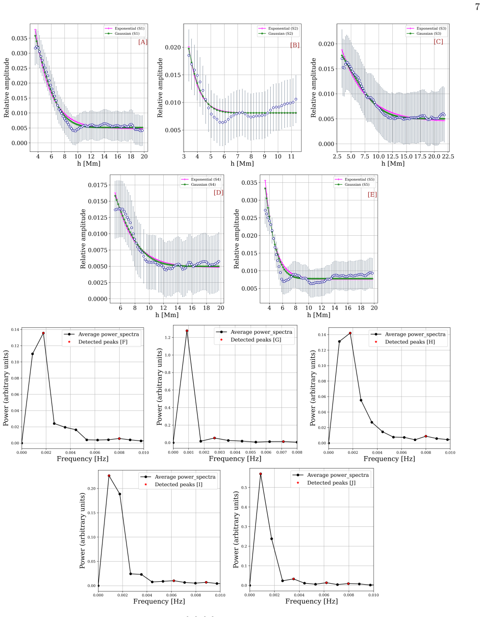
Time-distance maps are the central instrument: vertical slits convert the image sequence into maps where slanted bright and dark ridges trace outward-propagating compressive disturbances, and fitting Gaussian profiles along those ridges yields projected speeds. Transverse oscillations are extracted from contiguous horizontal slits by fitting a Gaussian across each plume substructure at every time step and then fitting the tracked centres with a sinusoid plus linear trend. The density diagnostic assumes kink-mode propagation and conserved wave energy flux, giving v proportional to rho^{-1/4}, which converts the measured velocity amplitudes into a relative electron-density profile with height.
What would settle it
Take simultaneous Doppler-velocity time-distance maps of the same plumes: if the 9-minute bright-dark ridge pattern appears with sinusoidal line-of-sight velocity oscillations at the same period, the slow-wave interpretation is confirmed; if the ridges correspond to non-oscillatory outflows with no periodic velocity signature, the longitudinal half of the coexistence claim fails.
Extended reading notes
Core claim
The central claim is the simultaneous, co-spatial presence of slow magneto-acoustic and Alfvénic waves in polar plumes, detected with a single instrument rather than by combining different telescopes. Ridge slopes in intensity time-distance maps give projected speeds of 115-125 km/s, amplitudes of 1.4-3.2% of background, and damping lengths of roughly 2.4-7.1 Mm, with a dominant period near 9.4 min in two plumes; the temperature implied by the sound speed is 0.58-0.69 MK. Gaussian and sinusoidal fits to transverse displacements in the same plumes yield log-normal means of 165±82 km displacement, 93±39 s period, and 12±7 km/s velocity amplitude, with displacement and velocity amplitudes incre
Load-bearing premise
The slanted ridges in the time-distance maps are taken to be slow magneto-acoustic waves; the paper itself notes that such propagating disturbances are often attributed to plasma outflows from jets or spicules, and no Doppler or multi-wavelength measurement is offered to rule that out.
Editorial extensions
If this is right
- A single EUI dataset can be used to study the energetics of both compressive and transverse wave modes in polar coronal holes, avoiding the plate-scale and cadence mismatches of combining different instruments.
- Compressive propagating disturbances are detectable not only in whole plumes but also in the fine-scale substructures inside them, indicating wave or flow organization at sub-plume scales.
- The measured transverse amplitude and velocity growth with height supports wave amplification in expanding plume geometry, though a larger sample is needed.
- The wave-derived plume temperatures of 0.58-0.69 MK provide a lower-limit temperature diagnostic based on the projected sound speed.
- The shorter damping lengths measured here compared with earlier AIA measurements are left as an open question, suggesting either stronger dissipation or an instrument-resolution effect.
Reading between the lines
- If the slow-wave identification is correct, the same data pipeline could be applied to inter-plume lanes, where longer-period compressive signatures have been reported, to see whether two-mode coexistence is a general property of open coronal structures.
- A simultaneous Doppler-velocity observation of the same plumes would settle whether the time-distance ridges are true slow waves or quasi-periodic outflows, a distinction imaging alone cannot make.
- Longer EUI campaigns could separate the 9.4 min signal from low-frequency leakage and test whether the unusually short damping lengths persist or are an artefact of the 19-minute window.
- The relative density profile inferred from transverse velocity amplitudes could be compared with density profiles from multi-wavelength EUV diagnostics, providing a direct cross-check of the energy-flux assumption.
Editorial analysis
A structured set of objections, weighed in public.
Referee Report
Summary. Using Solar Orbiter/EUI HRI_EUV 174 Å imaging from 14 September 2021, the paper reports the simultaneous presence of longitudinal ('slow magneto-acoustic') and transverse ('Alfvénic') oscillations in five polar plumes up to about 20 Mm. Longitudinal disturbances are identified as inclined bright/dark ridges in time–distance maps, with projected speeds of 115–125 km/s, relative amplitudes of 1.4–3.2%, damping lengths of about 2.4–7.1 Mm, and a 9.4-min periodicity reported for two of the five plumes; similar ridges are also seen in fine-scale substructures. Transverse oscillations are measured by manually fitting 98 Gaussian-determined centroid series, yielding log-normal mean displacement amplitude, period, and velocity amplitude. The paper concludes that this is the first co-spatial, co-temporal detection of both wave modes in the same polar plumes with Solar Orbiter/EUI.
Significance. If the longitudinal component is correctly identified as a slow magneto-acoustic wave, the result is a valuable observational advance: it demonstrates that a single high-resolution, high-cadence EUI dataset can capture both compressive and transverse MHD wave modes in the same coronal structures, with implications for wave heating and solar-wind acceleration. The paper also reports new detections in fine-scale plume substructures, which have not been emphasized before. Strengths include the use of state-of-the-art EUI data, manual fitting with propagated uncertainties, transparent descriptions of the fitting procedures, and publicly available data products. However, the significance of the central claim is conditional: the longitudinal-wave interpretation is not uniquely supported by the presented intensity imaging alone, given the well-known outflow alternative that the paper itself cites. The quantitative wave parameters (period, damping length, temperature) therefore also carry systematic uncertainties that are not fully reflected in the abstract and conclusions.
major comments (3)
- The identification of the inclined bright/dark ridges as slow magneto-acoustic waves is the load-bearing step for the coexistence claim. All reported supporting quantities—ridge slope (projected speed 115–125 km/s), intensity amplitude decay, and 9.4-min periodicity (in 2 of 5 slits)—are equally consistent with quasi-periodic plasma outflows or transient density-enhanced features. The Introduction (§1) itself notes that such disturbances 'are generally attributed to the outflows triggered by small-scale reconnection events, such as jets or spicules' (Pant et al. 2015; Jiao et al. 2015), and Appendix A identifies base brightenings and plasma ejections in the same slits. No Doppler, multi-temperature, or spectroscopic diagnostic is presented to rule out the outflow interpretation. Please provide such a test (e.g., simultaneous SPICE/EIS/CoMP velocities or a line-of-sight intensity-velocity
- [Abstract; §3.1.1(iii), Table 1] The abstract's 'periodicities of 9 min' is not supported for the full sample. Only Slits 1 and 3 show a 9.4-min peak; for Slits 2, 4, and 5 the dominant Fourier peak is at 18.8 min, equal to the total observing time, and the text concedes that these periods 'may be less reliable due to the short duration.' Because a periodicity is one of the few wave-like signatures that could distinguish an oscillation from a single outflow event, the absence of a detected period in 3/5 plumes should be stated in the abstract and Table 1 should mark these entries as non-detections rather than leaving the period column blank.
- [§3.1.1(ii)] The damping lengths in Table 1 are derived from Gaussian fits to the amplitude decay. However, for three of the five plumes the dominant period is longer than the 19-min observation window, so the fitted decay corresponds to less than one oscillation cycle. In this regime a Gaussian/exponential decay fit is essentially fitting the envelope of a single fading feature, not a wave damping length; the statement in §3.1.1(ii) that the Gaussian form is preferred for periodicities ≥ 20 min does not rescue this, since those periods are not actually measured. The values L_d = 2.45–7.16 Mm should be presented as amplitude-decay scale lengths, not wave damping lengths, unless a period is known.
minor comments (5)
- [Abstract; §3.2.3; §4 item 8] The log-normal means for displacement amplitude and period are inconsistent between §3.2.3 (165±82 km, 93±39 s) and Section 4 item 8 (174±91 km, 88±31 s). Please reconcile these values.
- [§3.1.1(iv)] The electron temperatures are acknowledged to be lower limits due to projection, but Table 1 reports only the small formal uncertainties propagated from the speed fits. Please quantify or explicitly state the systematic projection uncertainty.
- [§3.2.4, Fig. 6] The density power-law fit is written as ne(r)/ne,o = 63.06 h^-1.83, mixing r and h; please define the height variable and its units (Mm) and specify the normalization height clearly. Also describe whether the error bars are standard errors or scatter.
- [Fig. 2] The fitted ridges are indicated by cyan lines, but in several panels the ridges are faint; annotations or zoomed insets would help the reader verify the ridge selection and the discontinuities noted for Slit 4.
- [§1] The phrase 'Alfvénic waves' is used throughout; 'Alfvénic' should be 'Alfvénic' in the abstract and text. This is a typographical issue only.
Circularity Check
No significant circularity: the paper's wave parameters are direct measurements, and its temperature/density diagnostics use standard external relations rather than fitting the target claim.
full rationale
The paper contains no derivation step in which a prediction reduces by construction to its inputs. The slow-mode parameters are measured directly: ridge slopes give projected speeds (Section 3.1.1(i)), the amplitude and damping lengths come from Gaussian/exponential fits to the observed spatial amplitude profiles (Section 3.1.1(ii)), and the periods are taken from Fourier peaks of the time-distance maps (Section 3.1.1(iii)). The electron temperature is obtained from the standard relation c_s = 151 sqrt(T) after assuming the measured projected speed is the sound speed (Section 3.1.1(iv)); this is a diagnostic conversion under an explicit assumption, not a fitted input renamed as a prediction, and the paper itself labels the temperature a lower limit. The Alfvénic parameters follow from Gaussian center fitting plus sinusoidal fits (Section 3.2.1) and the density profile uses the external scaling v ∝ ρ^{-1/4} (Moran 2001; Weberg et al. 2020), not a model fitted to its own output. The self-citations (Shrivastav et al. 2024b, 2025; Krishna Prasad et al. 2012, 2019) are methodological references for fitting procedures, not load-bearing uniqueness theorems, and no ansatz is smuggled in via citation. The paper's own introduction notes that propagating disturbances in plumes are often attributed to outflows (Section 1, citing Pant et al. 2015 and Jiao et al. 2015), and the absence of Doppler/multi-wavelength data leaves the wave-versus-outflow interpretation open; however, that is an interpretive ambiguity and correctness risk, not a circular reduction. The central coexistence claim rests on independent detections of two wave signatures in the same structures, and no fitted constant is used to force that conclusion.
Assumptions & free parameters
free parameters (2)
- Density power-law coefficient =
63.06
- Density power-law exponent =
-1.83
assumptions (4)
- domain assumption The bright/dark ridges in time-distance maps are propagating compressive (slow magneto-acoustic) waves, not plasma outflows or unrelated intensity variations.
- domain assumption Transverse oscillation of the Gaussian-fitted intensity peak tracks kink-mode displacement of the plume.
- domain assumption Energy flux of the waves is conserved and BA (magnetic field times area) is constant with height, giving v proportional to n_e^-1/4.
- domain assumption Projected propagation speed equals the local sound speed (up to projection factor), allowing temperature T = (c_s/151)^2 MK.
Cite this review
Pith. "Pith review of Co-existence of longitudinal and transverse oscillations in polar plumes observed with Solar Orbiter/EUI." pith.science (2026). https://pith.science/paper/QX4Y5BNK
@misc{pith2026250907796,
  author       = {Pith},
  title        = {Pith review of: Co-existence of longitudinal and transverse oscillations in polar plumes observed with Solar Orbiter/EUI},
  year         = {2026},
  howpublished = {\url{https://pith.science/paper/QX4Y5BNK}},
  note         = {Machine review of arXiv:2509.07796}
}
abstract
Magnetohydrodynamic (MHD) waves play a key role in heating the solar corona and driving the solar wind. Recent observations have shown the presence of slow magneto-acoustic and Alfv\'enic waves in polar plumes and inter-plumes. However, a complete understanding of wave dynamics in the polar regions has long been limited by the lack of simultaneous, high-resolution observations. In this study, we utilize high spatial (210 km per pixel) and high cadence (5s) dataset from the Extreme Ultraviolet Imager (EUI) aboard Solar Orbiter, acquired on 14 September 2021. Our findings reveal the simultaneous presence of slow magneto-acoustic and Alfv\'enic waves within the same polar plumes. For slow magneto-acoustic waves, the amplitudes of propagating disturbances are 1.4 to 3.2$\%$ of background intensity, with periodicities of 9 min, and the projected speed of these disturbances ranges between 115 to 125 kms$^{-1}$. The corresponding electron temperature in plumes ranges between 0.58 and 0.69 MK. The damping length of these propagating disturbances for five plumes is $\approx$2.4 to 7.1 Mm. The propagating disturbances are also detected in the fine-scale substructures within the plumes. Alfv\'enic waves, on the other hand, are detected with average displacement amplitude, periodicity, and velocity amplitudes of 165$\pm$82 km, 93$\pm$39 s, and 12$\pm$7 kms$^{-1}$ respectively. The ranges for displacement amplitude, period, and velocity amplitude are 50-600 km, 50-250 s, and 3-32 kms$^{-1}$ respectively. These results mark the first demonstration of Solar Orbiter/EUI's ability to simultaneously detect both slow magneto-acoustic and Alfv\'enic wave modes extending up to 20 Mm in polar plumes.
Figures


Figures from the paper (4 more)


Reference graph
Works this paper leans on
-
[1]
1999, ApJ, 520, 880, doi: 10.1086/307502
Alexander, D. 1999, ApJ, 520, 880, doi: 10.1086/307502
doi:10.1086/307502 1999
-
[2]
2007, SoPh, 246, 3, doi: 10.1007/s11207-007-9029-z
Banerjee, D., Erd´ elyi, R., Oliver, R., & O’Shea, E. 2007, SoPh, 246, 3, doi: 10.1007/s11207-007-9029-z
-
[3]
Banerjee, D., O’Shea, E., & Doyle, J. G. 2000, SoPh, 196, 63, doi: 10.1023/A:1005265230456
-
[4]
Banerjee, D., O’Shea, E., Doyle, J. G., & Goossens, M. 2001, A&A, 377, 691, doi: 10.1051/0004-6361:20011153
-
[5]
Banerjee, D., P´ erez-Su´ arez, D., & Doyle, J. G. 2009, A&A, 501, L15, doi: 10.1051/0004-6361/200912242
-
[6]
Banerjee, D., Teriaca, L., Doyle, J. G., & Wilhelm, K. 1998, A&A, 339, 208
work page 1998
-
[7]
2021, SSRv, 217, 76, doi: 10.1007/s11214-021-00849-0
Banerjee, D., Krishna Prasad, S., Pant, V., et al. 2021, SSRv, 217, 76, doi: 10.1007/s11214-021-00849-0
-
[8]
2012, ApJ, 751, 110, doi: 10.1088/0004-637X/751/2/110
Bemporad, A., & Abbo, L. 2012, ApJ, 751, 110, doi: 10.1088/0004-637X/751/2/110
Show all 70 references
-
[9]
Zhugzhda, Y. D. 2011, ApJ, 728, 84, doi: 10.1088/0004-637X/728/2/84
2011 doi
-
[10]
Calabro, B., McAteer, R. T. J., & Bloomfield, D. S. 2013, SoPh, 286, 405, doi: 10.1007/s11207-013-0283-y
2013 doi
-
[11]
P., Huang, Z., D’Amicis, R., et al
Chitta, L. P., Huang, Z., D’Amicis, R., et al. 2025, A&A, 694, A71, doi: 10.1051/0004-6361/202452737
2025 doi
-
[12]
H., Bely-Dubau, F., et al
David, C., Gabriel, A. H., Bely-Dubau, F., et al. 1998, A&A, 336, L90 De Pontieu, B., Erd´ elyi, R., & De Moortel, I. 2005, ApJL, 624, L61, doi: 10.1086/430345 De Pontieu, B., & McIntosh, S. W. 2010, ApJ, 722, 1013, doi: 10.1088/0004-637X/722/2/1013 15 Figure 7.TD maps of the ...
1998 doi
-
[13]
E., & Gurman, J
DeForest, C. E., & Gurman, J. B. 1998, ApJL, 501, L217, doi: 10.1086/311460
1998 doi
-
[14]
E., Hoeksema, J
DeForest, C. E., Hoeksema, J. T., Gurman, J. B., et al. 1997, SoPh, 175, 393, doi: 10.1023/A:1004955223306
1997 doi
-
[15]
E., Lamy, P
DeForest, C. E., Lamy, P. L., & Llebaria, A. 2001, ApJ, 560, 490, doi: 10.1086/322497 Del Zanna, G., & Bromage, B. J. I. 1999, J. Geophys. Res., 104, 9753, doi: 10.1029/1998JA900067 Del Zanna, G., Bromage, B. J. I., & Mason, H. E. 2003, A&A, 398, 743, doi: 10.1051/0004-6361:20...
2001 doi
-
[16]
Domingo, V., Fleck, B., & Poland, A. I. 1995, SoPh, 162, 1, doi: 10.1007/BF00733425
1995 doi
-
[17]
G., Banerjee, D., & Perez, M
Doyle, J. G., Banerjee, D., & Perez, M. E. 1998, SoPh, 181, 91, doi: 10.1023/A:1005019931323
1998 doi
-
[18]
R., Schad, T
Fehlmann, A., Kuhn, J. R., Schad, T. A., et al. 2023, SoPh, 298, 5, doi: 10.1007/s11207-022-02098-y
2023 doi
-
[19]
L., & Handy, B
Freeland, S. L., & Handy, B. N. 1998, SoPh, 182, 497, doi: 10.1023/A:1005038224881
1998 doi
-
[20]
2024, A&A, 689, A195, doi: 10.1051/0004-6361/202450769
Karampelas, K. 2024, A&A, 689, A195, doi: 10.1051/0004-6361/202450769
2024 doi
-
[21]
Hahn, M., Landi, E., & Savin, D. W. 2012, ApJ, 753, 36, doi: 10.1088/0004-637X/753/1/36
2012 doi
-
[22]
N., Bruner, M
Handy, B. N., Bruner, M. E., Tarbell, T. D., et al. 1998, SoPh, 183, 29, doi: 10.1023/A:1005079622620
1998 doi
-
[23]
2015, ApJL, 809, L17, doi: 10.1088/2041-8205/809/1/L17
Jiao, F., Xia, L., Li, B., et al. 2015, ApJL, 809, L17, doi: 10.1088/2041-8205/809/1/L17
2015 doi
-
[24]
L., Esser, R., Gardner, L
Kohl, J. L., Esser, R., Gardner, L. D., et al. 1995, SoPh, 162, 313, doi: 10.1007/BF00733433 Krishna Prasad, S., Banerjee, D., & Gupta, G. R. 2011, A&A, 528, L4, doi: 10.1051/0004-6361/201016405 Krishna Prasad, S., Banerjee, D., & Singh, J. 2012, SoPh, 281, 67, doi: 10.1007/s1...
1995
-
[25]
2008, ApJ, 685, 1270, doi: 10.1086/591225
Landi, E. 2008, ApJ, 685, 1270, doi: 10.1086/591225
2008 doi
-
[26]
2023, ApJL, 952, L15, doi: 10.3847/2041-8213/ace423
Lim, D., Van Doorsselaere, T., Berghmans, D., et al. 2023, ApJL, 952, L15, doi: 10.3847/2041-8213/ace423
2023 doi
-
[27]
W., De Moortel, I., & Wang, Y
Liu, J., McIntosh, S. W., De Moortel, I., & Wang, Y. 2015, ApJ, 806, 273, doi: 10.1088/0004-637X/806/2/273
2015 doi
-
[28]
2018, ApJ, 856, 144, doi: 10.3847/1538-4357/aab42c
Magyar, N., & Van Doorsselaere, T. 2018, ApJ, 856, 144, doi: 10.3847/1538-4357/aab42c
2018 doi
-
[29]
2022, SolO/EUI Data Release 5.0 2022-04, https://doi.org/10.24414/2qfw-tr95
Mampaey, B., Verbeeck, F., Stegen, K., et al. 2022, SolO/EUI Data Release 5.0 2022-04, https://doi.org/10.24414/2qfw-tr95
2022 doi
-
[30]
2018, ApJ, 853, 134, doi: 10.3847/1538-4357/aaa1a3
Mandal, S., Krishna Prasad, S., & Banerjee, D. 2018, ApJ, 853, 134, doi: 10.3847/1538-4357/aaa1a3
2018 doi
-
[31]
P., Antolin, P., et al
Mandal, S., Chitta, L. P., Antolin, P., et al. 2022, A&A, 666, L2, doi: 10.1051/0004-6361/202244403
2022 doi
-
[32]
P., & de Moortel, I
McEwan, M. P., & de Moortel, I. 2006, A&A, 448, 763, doi: 10.1051/0004-6361:20054041
2006 doi
-
[33]
W., de Pontieu, B., Carlsson, M., et al
McIntosh, S. W., de Pontieu, B., Carlsson, M., et al. 2011, Nature, 475, 477, doi: 10.1038/nature10235
2011 doi
-
[34]
Nakariakov, V. M. 2024, MNRAS, 527, 5302, doi: 10.1093/mnras/stad3506
2024 doi
-
[35]
Moran, T. G. 2001, A&A, 374, L9, doi: 10.1051/0004-6361:20010643
2001 doi
-
[36]
J., Molnar, M., Cranmer, S
Morton, R. J., Molnar, M., Cranmer, S. R., & Schad, T. A. 2025a, ApJ, 982, 104, doi: 10.3847/1538-4357/adb8df
-
[37]
J., Tomczyk, S., & Pinto, R
Morton, R. J., Tomczyk, S., & Pinto, R. 2015, Nature Communications, 6, 7813, doi: 10.1038/ncomms8813
2015 doi
- [38]
-
[39]
M., Ofman, L., Deluca, E
Nakariakov, V. M., Ofman, L., Deluca, E. E., Roberts, B., & Davila, J. M. 1999, Science, 285, 862, doi: 10.1126/science.285.5429.862
1999 doi
-
[40]
Ofman, L., & Deforest, C. E. 2000, Advances in Space Research, 25, 1909, doi: 10.1016/S0273-1177(99)00622-5
2000 doi
-
[41]
M., & DeForest, C
Ofman, L., Nakariakov, V. M., & DeForest, C. E. 1999, ApJ, 514, 441, doi: 10.1086/306944
1999 doi
-
[42]
M., & Sehgal, N
Ofman, L., Nakariakov, V. M., & Sehgal, N. 2000a, ApJ, 533, 1071, doi: 10.1086/308691
-
[43]
Ofman, L., Romoli, M., Poletto, G., Noci, G., & Kohl, J. L. 1997, ApJL, 491, L111, doi: 10.1086/311067 —. 2000b, ApJ, 529, 592, doi: 10.1086/308252
1997 doi
-
[44]
2015, ApJ, 807, 71, doi: 10.1088/0004-637X/807/1/71
Pant, V., Dolla, L., Mazumder, R., et al. 2015, ApJ, 807, 71, doi: 10.1088/0004-637X/807/1/71
2015 doi
-
[45]
Pant, V., Magyar, N., Van Doorsselaere, T., & Morton, R. J. 2019, ApJ, 881, 95, doi: 10.3847/1538-4357/ab2da3
2019 doi
-
[46]
2017, ApJL, 847, L5, doi: 10.3847/2041-8213/aa880f
Pant, V., Tiwari, A., Yuan, D., & Banerjee, D. 2017, ApJL, 847, L5, doi: 10.3847/2041-8213/aa880f
2017 doi
-
[47]
2020, ApJ, 899, 1, doi: 10.3847/1538-4357/aba429
Pant, V., & Van Doorsselaere, T. 2020, ApJ, 899, 1, doi: 10.3847/1538-4357/aba429
2020 doi
-
[48]
D., Thompson, B
Pesnell, W. D., Thompson, B. J., & Chamberlin, P. C. 2012, SoPh, 275, 3, doi: 10.1007/s11207-011-9841-3
2012 doi
-
[49]
2023, ApJ, 946, 36, doi: 10.3847/1538-4357/acb26a
Berghmans, D. 2023, ApJ, 946, 36, doi: 10.3847/1538-4357/acb26a
2023 doi
-
[50]
2015, Living Reviews in Solar Physics, 12, 7, doi: 10.1007/lrsp-2015-7
Poletto, G. 2015, Living Reviews in Solar Physics, 12, 7, doi: 10.1007/lrsp-2015-7
2015 doi
-
[51]
R., Warner, M., Keil, S
Rimmele, T. R., Warner, M., Keil, S. L., et al. 2020, SoPh, 295, 172, doi: 10.1007/s11207-020-01736-7
2020 doi
-
[52]
2019, MHD waves in the solar atmosphere
Roberts, B. 2019, MHD waves in the solar atmosphere
2019
-
[53]
2020, A&A, 642, A8, doi: 10.1051/0004-6361/201936663
Rochus, P., Auch` ere, F., Berghmans, D., et al. 2020, A&A, 642, A8, doi: 10.1051/0004-6361/201936663
2020 doi
-
[54]
Saba, J. L. R., & Strong, K. T. 1991, ApJ, 375, 789, doi: 10.1086/170243
1991 doi
-
[55]
2015, ApJL, 815, L16, doi: 10.1088/2041-8205/815/1/L16
Samanta, T., Pant, V., & Banerjee, D. 2015, ApJL, 815, L16, doi: 10.1088/2041-8205/815/1/L16
2015 doi
-
[56]
K., Pant, V., & Antolin, P
Shrivastav, A. K., Pant, V., & Antolin, P. 2024a, A&A, 689, A295, doi: 10.1051/0004-6361/202449677
-
[57]
K., Pant, V., Kumar, R., et al
Shrivastav, A. K., Pant, V., Kumar, R., et al. 2025, ApJ, 979, 6, doi: 10.3847/1538-4357/ad95fb
2025 doi
-
[58]
K., Pant, V., Berghmans, D., et al
Shrivastav, A. K., Pant, V., Berghmans, D., et al. 2024b, A&A, 685, A36, doi: 10.1051/0004-6361/202346670
-
[59]
J., Samanta, T., & Van Doorsselaere, T
Skirvin, S. J., Samanta, T., & Van Doorsselaere, T. 2024, A&A, 689, A135, doi: 10.1051/0004-6361/202450186
2024 doi
-
[60]
W., & Bethge, C
Threlfall, J., De Moortel, I., McIntosh, S. W., & Bethge, C. 2013, A&A, 556, A124, doi: 10.1051/0004-6361/201321782
2013 doi
-
[61]
O., Morton, R
Thurgood, J. O., Morton, R. J., & McLaughlin, J. A. 2014, ApJL, 790, L2, doi: 10.1088/2041-8205/790/1/L2
2014 doi
-
[62]
W., Habbal, S
Tian, H., McIntosh, S. W., Habbal, S. R., & He, J. 2011, ApJ, 736, 130, doi: 10.1088/0004-637X/736/2/130
2011 doi
-
[63]
W., Wang, T., et al
Tian, H., McIntosh, S. W., Wang, T., et al. 2012, ApJ, 759, 144, doi: 10.1088/0004-637X/759/2/144
2012 doi
-
[64]
W., Keil, S
Tomczyk, S., McIntosh, S. W., Keil, S. L., et al. 2007, Science, 317, 1192, doi: 10.1126/science.1143304
2007 doi
-
[65]
L., Darnell, T., et al
Tomczyk, S., Card, G. L., Darnell, T., et al. 2008, SoPh, 247, 411, doi: 10.1007/s11207-007-9103-6
2008 doi
-
[66]
K., Prasad, S
Tripathy, S. K., Prasad, S. K., & Banerjee, D. 2025, Properties of slow magneto-acoustic waves observed simultaneously using Hi-C 2.1 and AIA. https://arxiv.org/abs/2506.06126 Van Doorsselaere, T., Nakariakov, V. M., & Verwichte, E. 2008, ApJL, 676, L73, doi: 10.1086/587029 17...
2025 arXiv
-
[67]
J., Morton, R
Weberg, M. J., Morton, R. J., & McLaughlin, J. A. 2018, ApJ, 852, 57, doi: 10.3847/1538-4357/aa9e4a —. 2020, ApJ, 894, 79, doi: 10.3847/1538-4357/ab7c59
2018 doi
-
[68]
2006, A&A, 455, 697, doi: 10.1051/0004-6361:20054693
Wilhelm, K. 2006, A&A, 455, 697, doi: 10.1051/0004-6361:20054693
2006 doi
-
[69]
1998, SSRv, 85, 371, doi: 10.1023/A:1005187509676
Wilhelm, K., & Bodmer, R. 1998, SSRv, 85, 371, doi: 10.1023/A:1005187509676
1998 doi
-
[70]
P., et al
Zouganelis, I., De Groof, A., Walsh, A. P., et al. 2020, A&A, 642, A3, doi: 10.1051/0004-6361/202038445
2020 doi
Reviewed August 4, 2026 · model on record in the stance chip above.
Discussion (0). Continue with ORCID to comment.