Multiscaling in Wasserstein Spaces
Pith reviewed 2026-05-18 17:23 UTC · model grok-4.3
The pith
A multiscale transform for Wasserstein measures preserves geodesics via McCann interpolants and introduces an optimality number for scale-wise deviation measurement.
A machine-rendered reading of the paper's core claim, the machinery that carries it, and where it could break.
Core claim
We construct a multiscale transform applicable to both absolutely continuous and discrete measures. Central to our approach is a refinement operator based on McCann's interpolants, which preserves the geodesic structure of measure flows and serves as an upsampling mechanism. Building on this, we introduce the optimality number, a scalar that quantifies deviations of a sequence from Wasserstein geodesicity across scales.
What carries the argument
The refinement operator based on McCann's interpolants, which acts as an upsampling mechanism that preserves geodesic structure in measure flows, enabling the multiscale transform and the computation of the optimality number.
If this is right
- The multiscale transform is stable.
- Coefficients exhibit geometric decay.
- It enables denoising and anomaly detection in Gaussian flows.
- Point cloud dynamics under vector fields can be analyzed at multiple scales.
- Neural network learning trajectories admit a multiscale characterization.
Where Pith is reading between the lines
- The optimality number might serve as a general diagnostic for irregular dynamics in measure-valued time series from any source.
- The same refinement construction could extend to other optimal transport metrics if an analogous interpolant exists.
- Applications to fluid simulations or population dynamics would test whether the geometric decay holds in practice.
- Connecting the optimality number to classical irregularity measures in dynamical systems could link this work to existing anomaly tools.
Load-bearing premise
The refinement operator based on McCann's interpolants preserves the geodesic structure of measure flows for arbitrary sequences of measures and can be used as a stable upsampling mechanism without introducing artifacts that affect the optimality number at finer scales.
What would settle it
Apply the refinement operator to a sequence of discrete measures known to deviate from a Wasserstein geodesic, then recompute the optimality number at the finer scales; an unexpected increase due to the operator itself would show that artifacts are introduced.
Figures


read the original abstract
We present a novel multiscale framework for analyzing sequences of probability measures in Wasserstein spaces over Euclidean domains. Exploiting the intrinsic geometry of optimal transport, we construct a multiscale transform applicable to both absolutely continuous and discrete measures. Central to our approach is a refinement operator based on McCann's interpolants, which preserves the geodesic structure of measure flows and serves as an upsampling mechanism. Building on this, we introduce the optimality number, a scalar that quantifies deviations of a sequence from Wasserstein geodesicity across scales, enabling the detection of irregular dynamics and anomalies. We establish key theoretical guarantees, including stability of the transform and geometric decay of coefficients, ensuring robustness and interpretability of the multiscale representation. Finally, we demonstrate the versatility of our methodology through numerical experiments: denoising and anomaly detection in Gaussian flows, analysis of point cloud dynamics under vector fields, and the multiscale characterization of neural network learning trajectories.
Editorial analysis
A structured set of objections, weighed in public.
Referee Report
Summary. The paper constructs a multiscale transform for sequences of probability measures in Wasserstein spaces over Euclidean domains, applicable to both absolutely continuous and discrete measures. It introduces a refinement operator based on McCann interpolants that is claimed to preserve geodesic structure and function as stable upsampling, defines an optimality number to quantify deviations from Wasserstein geodesicity across scales, establishes stability of the transform together with geometric decay of coefficients, and illustrates the framework via numerical experiments on denoising/anomaly detection in Gaussian flows, point-cloud dynamics, and neural-network learning trajectories.
Significance. If the central claims hold, the work supplies a new scalar diagnostic (the optimality number) and an upsampling mechanism grounded in optimal transport geometry that could be useful for detecting irregular dynamics in measure-valued sequences. The extension to discrete measures and the reported geometric decay would be concrete strengths if the proofs are robust to non-uniqueness of couplings.
major comments (2)
- [§3.2] §3.2 (refinement operator): The construction uses McCann interpolants along optimal plans, but for discrete measures the optimal coupling is frequently non-unique. The manuscript does not specify a canonical selection rule nor prove that the optimality number is invariant under different choices of the coupling. This directly affects the claim that the operator preserves geodesic structure for arbitrary sequences and serves as a stable upsampling mechanism without introducing scale-dependent artifacts.
- [Theorem 5.3] Theorem 5.3 (geometric decay): The decay estimate for the optimality-number coefficients is stated to hold uniformly, yet it appears to rest on the refinement operator being well-defined and geodesic-preserving for discrete measures. If different couplings produce different interpolated measures at intermediate scales, the decay rate may depend on the (unspecified) choice and the theorem would require an additional invariance argument.
minor comments (2)
- [§4] Notation for the optimality number is introduced without an explicit formula in the main text; a displayed equation would improve readability.
- [Figure 4] Figure 4 (point-cloud experiment) lacks error bars or multiple random seeds; the reported optimality numbers appear sensitive to initialization.
Simulated Author's Rebuttal
We thank the referee for the careful reading and constructive comments on the refinement operator and the geometric decay result. We address the two major comments point by point below and will revise the manuscript accordingly to strengthen the treatment of discrete measures.
read point-by-point responses
-
Referee: [§3.2] §3.2 (refinement operator): The construction uses McCann interpolants along optimal plans, but for discrete measures the optimal coupling is frequently non-unique. The manuscript does not specify a canonical selection rule nor prove that the optimality number is invariant under different choices of the coupling. This directly affects the claim that the operator preserves geodesic structure for arbitrary sequences and serves as a stable upsampling mechanism without introducing scale-dependent artifacts.
Authors: We agree that non-uniqueness of optimal couplings must be handled explicitly for discrete measures. The current manuscript assumes an optimal plan exists but does not detail a selection procedure. In the revision we will add a canonical selection rule in §3.2 (for example, the coupling obtained as the zero-temperature limit of entropic optimal transport, or the one minimizing a secondary quadratic cost among all optimal plans). We will also insert a short invariance lemma showing that the optimality number depends only on the Wasserstein distances between the interpolated marginals and is therefore independent of the particular choice of optimal coupling. revision: yes
-
Referee: [Theorem 5.3] Theorem 5.3 (geometric decay): The decay estimate for the optimality-number coefficients is stated to hold uniformly, yet it appears to rest on the refinement operator being well-defined and geodesic-preserving for discrete measures. If different couplings produce different interpolated measures at intermediate scales, the decay rate may depend on the (unspecified) choice and the theorem would require an additional invariance argument.
Authors: We acknowledge that the proof of Theorem 5.3 implicitly relies on the refinement operator being unambiguously defined. The revised manuscript will include the invariance lemma mentioned above and will use it to show that the coefficients entering the geometric decay bound are the same for any choice of optimal coupling. With this addition the uniform decay statement remains valid for both absolutely continuous and discrete measures. revision: yes
Circularity Check
Derivation self-contained from Wasserstein geometry and McCann interpolants
full rationale
The paper constructs the multiscale transform and optimality number directly from the intrinsic geometry of optimal transport and McCann's interpolants, which are standard external results. No equation reduces the optimality number to a fitted parameter by construction, no self-citation chain bears the central load, and the refinement operator is asserted to preserve geodesicity without the claim itself being defined in terms of the output scalar. The framework supplies independent stability guarantees and numerical validation, making the derivation non-circular.
Axiom & Free-Parameter Ledger
axioms (1)
- domain assumption McCann's interpolants preserve geodesic structure in the Wasserstein space for sequences of measures
invented entities (1)
-
optimality number
no independent evidence
Lean theorems connected to this paper
-
IndisputableMonolith/Cost/FunctionalEquation.leanwashburn_uniqueness_aczel unclear?
unclearRelation between the paper passage and the cited Recognition theorem.
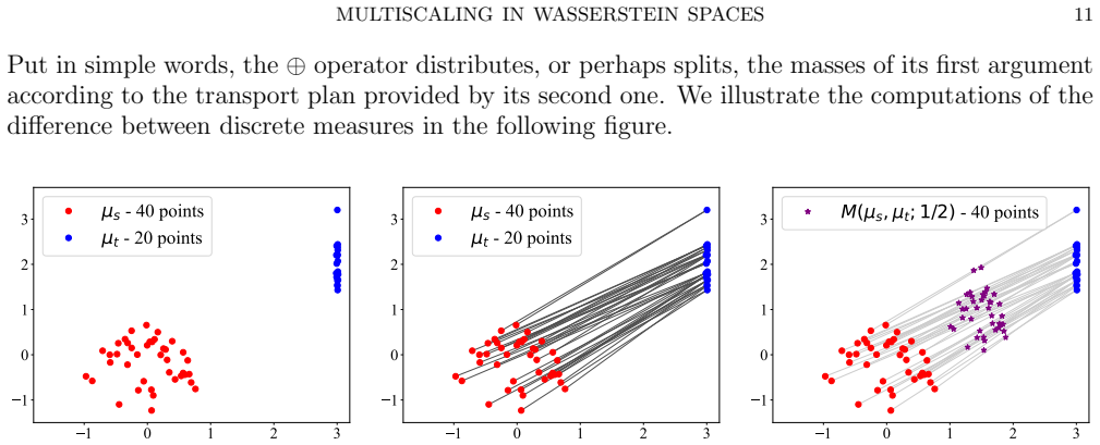
Central to our approach is a refinement operator based on McCann's interpolants, which preserves the geodesic structure of measure flows and serves as an upsampling mechanism... optimality number, a scalar that quantifies deviations of a sequence from Wasserstein geodesicity across scales
What do these tags mean?
- matches
- The paper's claim is directly supported by a theorem in the formal canon.
- supports
- The theorem supports part of the paper's argument, but the paper may add assumptions or extra steps.
- extends
- The paper goes beyond the formal theorem; the theorem is a base layer rather than the whole result.
- uses
- The paper appears to rely on the theorem as machinery.
- contradicts
- The paper's claim conflicts with a theorem or certificate in the canon.
- unclear
- Pith found a possible connection, but the passage is too broad, indirect, or ambiguous to say the theorem truly supports the claim.
Reference graph
Works this paper leans on
-
[1]
Barycenters in the Wasserstein space.SIAM Journal on Mathematical Analysis, 43(2):904–924, 2011
Martial Agueh and Guillaume Carlier. Barycenters in the Wasserstein space.SIAM Journal on Mathematical Analysis, 43(2):904–924, 2011
work page 2011
-
[2]
Springer Science & Business Media, 2008
Luigi Ambrosio, Nicola Gigli, and Giuseppe Savar´ e.Gradient flows: in metric spaces and in the space of probability measures. Springer Science & Business Media, 2008
work page 2008
-
[3]
Jean Baccou and Jacques Liandrat. Subdivision scheme for discrete probability measure- valued data.Applied Mathematics Letters, 158:109233, 2024
work page 2024
-
[4]
Efficient trajectory inference in Wasserstein space using consecutive averaging
Amartya Banerjee, Harlin Lee, Nir Sharon, and Caroline Moosm¨ uller. Efficient trajectory inference in Wasserstein space using consecutive averaging. InThe 28th International Con- ference on Artificial Intelligence and Statistics, 2025
work page 2025
-
[5]
Statistical data analysis in the Wasserstein space.ESAIM: Proceedings and Surveys, 68:1–19, 2020
J´ er´ emie Bigot. Statistical data analysis in the Wasserstein space.ESAIM: Proceedings and Surveys, 68:1–19, 2020
work page 2020
-
[6]
Yanshuo Chen, Zhengmian Hu, Wei Chen, and Heng Huang. Fast and scalable Wasserstein-1 neural optimal transport solver for single-cell perturbation prediction.Bioinformatics, 41(Sup- plement 1):i513–i522, 2025
work page 2025
-
[7]
Wasserstein regression.Journal of the American Statistical Association, 118(542):869–882, 2023
Yaqing Chen, Zhenhua Lin, and Hans-Georg M¨ uller. Wasserstein regression.Journal of the American Statistical Association, 118(542):869–882, 2023
work page 2023
-
[8]
Fast and smooth interpolation on Wasserstein space
Sinho Chewi, Julien Clancy, Thibaut Le Gouic, Philippe Rigollet, George Stepaniants, and Austin Stromme. Fast and smooth interpolation on Wasserstein space. InInternational Conference on Artificial Intelligence and Statistics, pages 3061–3069. PMLR, 2021
work page 2021
- [9]
-
[10]
Pinar Demetci, Rebecca Santorella, Bj¨ orn Sandstede, William Stafford Noble, and Ritambhara Singh. Gromov-Wasserstein optimal transport to align single-cell multi-omics data.BioRxiv, pages 2020–04, 2020
work page 2020
-
[11]
The MNIST database of handwritten digit images for machine learning research
Li Deng. The MNIST database of handwritten digit images for machine learning research. IEEE signal processing magazine, 29(6):141–142, 2012
work page 2012
-
[12]
David L Donoho. Interpolating wavelet transforms.Preprint, Department of Statistics, Stan- ford University, 2(3):1–54, 1992. 24 W. MATTAR AND N. SHARON
work page 1992
-
[13]
David C. Dowson and Basil V. Landau. The Fr´ echet distance between multivariate normal distributions.Journal of multivariate analysis, 12(3):450–455, 1982
work page 1982
-
[14]
Subdivision schemes in CAGD.Advances in numerical analysis, 2:36–104, 1992
Nira Dyn. Subdivision schemes in CAGD.Advances in numerical analysis, 2:36–104, 1992
work page 1992
-
[15]
Subdivision schemes in geometric modelling.Acta Numerica, 11:73–144, 2002
Nira Dyn and David Levin. Subdivision schemes in geometric modelling.Acta Numerica, 11:73–144, 2002
work page 2002
-
[16]
Nira Dyn and Nir Sharon. Manifold-valued subdivision schemes based on geodesic inductive averaging.Journal of Computational and Applied Mathematics, 311:54–67, 2017
work page 2017
-
[17]
Subdivision schemes in metric spaces.preprint arXiv:2509.08070, 2025
Nira Dyn and Nir Sharon. Subdivision schemes in metric spaces.preprint arXiv:2509.08070, 2025
-
[18]
Nira Dyn and Xiaosheng Zhuang. Linear multiscale transforms based on even-reversible subdi- vision operators.Excursions in Harmonic Analysis, Volume 6: In Honor of John Benedetto’s 80th Birthday, pages 297–319, 2021
work page 2021
-
[19]
Jianing Fan and Hans-Georg M¨ uller. Conditional Wasserstein barycenters and interpola- tion/extrapolation of distributions.IEEE Transactions on Information Theory, 2024
work page 2024
-
[20]
Philipp Grohs. Stability of manifold-valued subdivision schemes and multiscale transforma- tions.Constructive approximation, 32:569–596, 2010
work page 2010
-
[21]
Improved training of Wasserstein gans.Advances in neural information processing systems, 30, 2017
Ishaan Gulrajani, Faruk Ahmed, Martin Arjovsky, Vincent Dumoulin, and Aaron C Courville. Improved training of Wasserstein gans.Advances in neural information processing systems, 30, 2017
work page 2017
-
[22]
Manifold learning in Wasserstein space.SIAM Journal on Mathematical Analysis, 57(3):2983–3029, 2025
Keaton Hamm, Caroline Moosm¨ uller, Bernhard Schmitzer, and Matthew Thorpe. Manifold learning in Wasserstein space.SIAM Journal on Mathematical Analysis, 57(3):2983–3029, 2025
work page 2025
-
[23]
Dominik Klein, Th´ eo Uscidda, Fabian Theis, and Marco Cuturi. GENOT: Entropic (Gromov) Wasserstein flow matching with applications to single-cell genomics.Advances in Neural Information Processing Systems, 37:103897–103944, 2024
work page 2024
-
[24]
Jeffrey M Lane and Richard F Riesenfeld. A theoretical development for the computer gener- ation and display of piecewise polynomial surfaces.IEEE Transactions on Pattern Analysis and Machine Intelligence, pages 35–46, 1980
work page 1980
-
[25]
Pyramid transform of manifold data via subdivision operators
Wael Mattar and Nir Sharon. Pyramid transform of manifold data via subdivision operators. IMA Journal of Numerical Analysis, 43(1):387–413, 2023
work page 2023
-
[26]
A convexity principle for interacting gases.Advances in mathematics, 128(1):153–179, 1997
Robert J McCann. A convexity principle for interacting gases.Advances in mathematics, 128(1):153–179, 1997
work page 1997
-
[27]
The geometry of dissipative evolution equations: The porous medium equation
Felix Otto. The geometry of dissipative evolution equations: The porous medium equation. Communications in Partial Differential Equations, 26(1-2):101–174, 2001
work page 2001
-
[28]
Victor M Panaretos and Yoav Zemel.An invitation to statistics in Wasserstein space. Springer Nature, 2020
work page 2020
-
[29]
Gabriel Peyr´ e, Marco Cuturi, et al. Computational optimal transport: With applications to data science.Foundations and Trends in Machine Learning, 11(5-6):355–607, 2019
work page 2019
-
[30]
Wasserstein barycenter and its application to texture mixing
Julien Rabin, Gabriel Peyr´ e, Julie Delon, and Marc Bernot. Wasserstein barycenter and its application to texture mixing. InInternational conference on scale space and variational methods in computer vision, pages 435–446. Springer, 2011
work page 2011
-
[31]
Inam Ur Rahman, Iddo Drori, Victoria C Stodden, David L Donoho, and Peter Schr¨ oder. Mul- tiscale representations for manifold-valued data.Multiscale Modeling & Simulation, 4(4):1201– 1232, 2005
work page 2005
-
[32]
Introduction to Optimal Transport Theory
Filippo Santambrogio. Introduction to optimal transport theory.preprint arXiv:1009.3856, 2010
work page internal anchor Pith review Pith/arXiv arXiv 2010
-
[33]
Optimal transport for applied mathematicians.Birk¨ auser, NY, 55(58- 63):94, 2015
Filippo Santambrogio. Optimal transport for applied mathematicians.Birk¨ auser, NY, 55(58- 63):94, 2015. MULTISCALING IN W ASSERSTEIN SPACES 25
work page 2015
-
[34]
Geoffrey Schiebinger, Jian Shu, Marcin Tabaka, Brian Cleary, Vidya Subramanian, Aryeh Solomon, Joshua Gould, Siyan Liu, Stacie Lin, Peter Berube, et al. Optimal-transport analysis of single-cell gene expression identifies developmental trajectories in reprogramming.Cell, 176(4):928–943, 2019
work page 2019
-
[35]
American Mathematical Soc., 2021
C´ edric Villani.Topics in optimal transportation, volume 58. American Mathematical Soc., 2021
work page 2021
-
[36]
Geometric subdivision and multiscale transforms
Johannes Wallner. Geometric subdivision and multiscale transforms. InHandbook of Varia- tional Methods for Nonlinear Geometric Data, pages 121–152. Springer, 2020
work page 2020
-
[37]
Yunan Yang, Bj¨ orn Engquist, Junzhe Sun, and Brittany F Hamfeldt. Application of opti- mal transport and the quadratic Wasserstein metric to full-waveform inversion.Geophysics, 83(1):R43–R62, 2018. Appendix We prove the inequalities (38). Letµ, ν∈ P p(Rd) for somep >1 andψ, eψ:R d →R d be two measurable Lipschitz maps. We have Wp(ψ#µ,eψ#µ)≤ ∥ψ− eψ∥Lp(µ) ...
work page 2018
discussion (0)
Sign in with ORCID, Apple, or X to comment. Anyone can read and Pith papers without signing in.