REVIEW 4 major objections 4 minor 43 references
Compressed Bayesian Tensor Regression
T0 review · 4 major / 4 minor · reviewed 2026-08-04 · deepseek-v4-flash
Pith's one-line read Compressed Bayesian tensor regression projects high-dimensional tensor covariates into a small subspace and predicts out-of-sample at least as well as—often better than—the full tensor regression, with far lower cost.
desk verdict GTRP is a sensible extension and the real-data gains are real, but the JL-type theory is mis-normalized and needs major repair before the paper's central claims can be trusted. read the letter →
The pith
A machine-rendered reading of the paper's core claim, the machinery that carries it, and where it could break.
The reading
What carries the argument
The key identity is the distance-preservation bound for GTRP: for all U,V, (1−ε)||U−V||² ≤ ||√(p(N)/q(M))GTRP(U−V)||² ≤ (1+ε)||U−V||² with probability at least 1−n^{−β}, provided q(M) is large enough. This is what connects the compressed covariates to the original signal. The second piece is the hierarchical low-rank prior B = Σ_d γ_1^{(d)}∘...∘γ_M^{(d)} with shrinkage scales, which makes the Gibbs updates closed-form; and Bayesian model averaging over L random projections addresses the variability introduced by any single projection.
What would settle it
Generate a fixed tensor A with a single 1 and zeros elsewhere, sample many projection matrices/tensors from Eq. (5), and compute ||√(p(N)/q(M))GTRP(A)||². Its average is p(N), not 1; for p(N)>1 this contradicts the claimed (1±ε) bound around ||A||². A reader can see this directly from the second moment calculation in the proof of Theorem 1.
Extended reading notes
Core claim
The central object is the Generalized Tensor Random Projection (GTRP), which maps an order-N covariate tensor to a smaller order-M tensor by mode-wise products with sparse random matrices along some modes and a tensor-wise product with a random projection tensor along the rest. The paper proves that, with scaling √(p(N)/q(M)), squared distances between any two projected tensors are preserved within 1±ε with high probability once the compressed dimension is large enough, and it proves posterior consistency for the tensor coefficient under both a tensor-normal prior and a low-rank parallel-factor prior. A closed-form Gibbs sampler approximates the posterior of the low-rank compressed model. Th
Load-bearing premise
The load-bearing premise is that the scaling √(p(N)/q(M)) makes GTRP norm-preserving in expectation; with the paper's unit-variance projection entries, the expected squared distance is multiplied by p(N), so the concentration inequalities as stated hold only after an additional 1/√p(N) rescaling.
Editorial extensions
If this is right
- Tensor regressions that were previously infeasible because of the size of the covariate array become tractable: project first, then run the Gibbs sampler on the small compressed tensor.
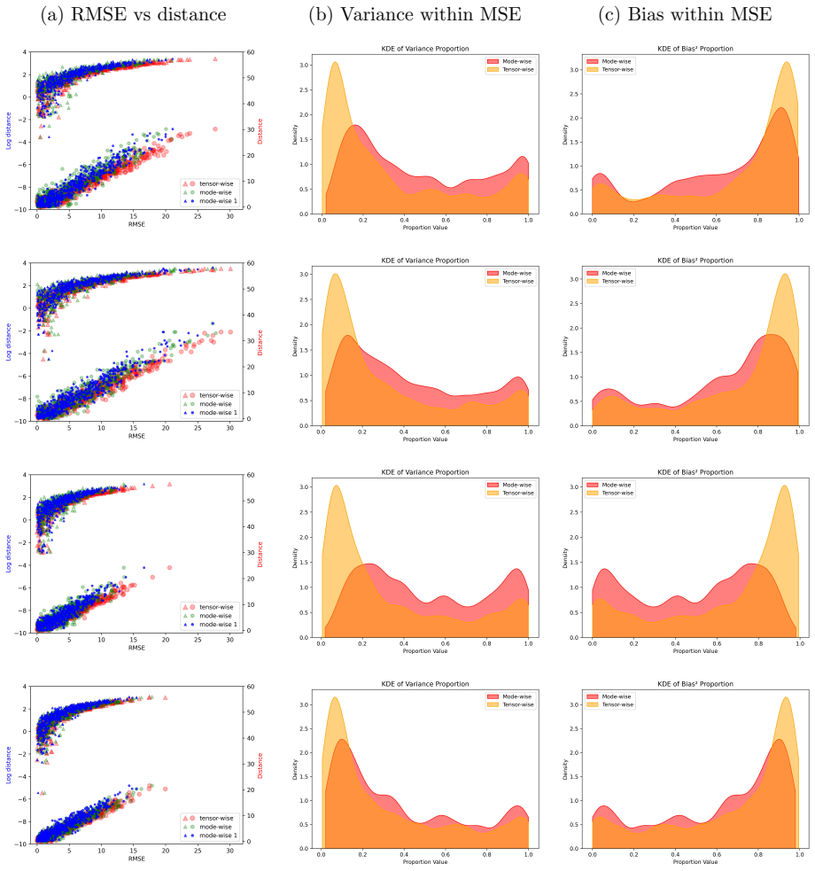
- Mode-preserving projections should be preferred in practice; the simulations and the financial application show they predict better than projections that flatten the tensor.
- Averaging over several random projections brings the method close to the stability of the uncompressed fit, removing dependence on a single projection draw.
- The posterior consistency theorems say that as n grows, the compressed-model predictive distribution converges to the truth, so the compression does not silently destroy inferential validity.
- In the reported 60×60 simulation with 2,000 observations, the compressed model runs roughly two orders of magnitude faster than the uncompressed Bayesian tensor regression while achieving lower out-of-sample RMSE.
Reading between the lines
- A corrected normalization (e.g., scaling by 1/√q(M) or drawing projection entries with variance 1/p(N)) would restore the literal distance-preservation inequalities; because a global rescaling of covariates can be absorbed by the regression coefficients, the paper's predictive conclusions would likely survive the fix.
- The GTRP framework could be pushed beyond prediction: if the projection is designed to be nearly invertible on low-rank tensors, the posterior for the compressed coefficient could be used to recover the support or structure of the original coefficient tensor; the paper does not explore this.
- A natural next experiment is to let Bayesian model averaging mix over projection types (tensor-wise vs mode-wise) rather than only over matrices of the same type; the paper's simulations show type choice is the largest performance lever.
- The consistency rate ε_n = n^{δ}, δ<0, with compressed dimension growing sublinearly in n, suggests a direct empirical check: tracking predictive error as n and q grow should show the predicted contraction; that would test whether the theoretical rate is tight.
Editorial analysis
A structured set of objections, weighed in public.
Referee Report
Summary. The paper proposes a Compressed Bayesian Tensor Regression (CBTR) framework in which tensor-valued covariates are mapped by a Generalized Tensor Random Projection (GTRP) into a lower-dimensional tensor, combined with a hierarchical PARAFAC prior, a closed-form Gibbs sampler, and Bayesian model averaging over random projections. The main theoretical claims are JL-type concentration inequalities for GTRP (Prop. 1, Thm. 1, Thm. 2) and posterior consistency of the predictive density (Thm. 3, Thm. 4). The method is evaluated through extensive simulations and a financial application.
Significance. If the theoretical claims were valid, this would be a useful contribution to high-dimensional tensor regression: the GTRP framework is flexible, the Gibbs sampler is explicit, and the simulation study and real-data application are substantial. However, the central concentration inequalities are mis-scaled, and the posterior consistency theorems inherit the same normalization problem. The advertised 'strong theoretical support' does not hold as stated, so the paper's main formal contribution is currently unsupported.
major comments (4)
- [Sec. 2.2, Eq. (2), Eq. (5), Prop. 1, Thm. 1] The map f is not norm-preserving. The entries in (5) have variance 1. For any fixed A, E[GTRP(A)_i^2] = ||A||^2; summing over q(M) output entries gives E||GTRP(A)||^2 = q(M)||A||^2. Since f(X) = sqrt(c) GTRP(X) with c = p(N)/q(M), E||f(A)||^2 = p(N)||A||^2, not ||A||^2. Thus the claimed (1±epsilon) preservation cannot hold for p(N) > 1. The correct normalization would be f = GTRP/sqrt(q(M)) (or equivalent), which changes the theorem statements and subsequent proofs.
- [Appendix A.2, Lemma 1] The Gaussian comparison is reversed. For Q in (A.1), Q_{i1...iN} = (1/sqrt(p(N))) sum_{j1...jN} prod H_{m,j_m,i_m}; the sum contains p(N) independent zero-mean unit-variance terms, so E(Q^2) = 1. For T, E(T^2) = prod(1/p_m) = 1/p(N). Hence E(Q^2) <= E(T^2) fails for k=1. Lemma 3 and the upper-tail bound inherit this error. The lower-tail inequality (A.43) also uses E(Q^2) = 1/p(N), contradicting Lemma 1. The proof of Theorem 1 is therefore invalid.
- [Sec. 4, Assumption A.3, Thms. 3 and 4] Assumption A.3 asserts that the norm condition is satisfied with high probability 'as described in Proposition 1 and Theorem 1'. Since those results are false without renormalization, the justification for A.3 collapses. In the proof of Theorem 3 (Appendix A.4, condition (c)), the lower bound on prior mass uses Var(<GTRP(X),B>) proportional to ||GTRP(X)||^2; without a valid normalized projection, this bound is not established. Theorem 4 relies on the same assumptions through A.4. Thus the posterior consistency results are unsupported as stated.
- [Appendix A.3, proof of Thm. 2] The proof redefines f(X) as (1/sqrt(q(N))) <H_{1,:,i1} o ... o H_{N,:,iN}, X>, whereas Section 2.2 defines f(X) = sqrt(p(N)/q(N)) GTRP(X). Since a GTRP entry equals that inner product, the factor is inconsistent; this changes the variance computation and the resulting bound. The normalization problem is systemic rather than a local typo.
minor comments (4)
- [Eq. (20)] The efficiency score formula should read 1/(RMSE x Cost); as printed, '1 RMSE x Cost' is ambiguous.
- [Sec. 5.1] The statement 'This required 2560 simulations for a given psi' is not justified from the described designs; please clarify the counting.
- [Thm. 1] The phrase 'Assume a sequence ... satisfy q(N) >= q0 with probability at least 1 - n^{-beta}' is unclear: q is a chosen dimension, not a random quantity. Rephrase to separate the choice of q from the probability over projections.
- [Sec. 2.3] The prior in (9) is written for B in R^{p1 x ... x pM}, but after compression B should be in R^{q1 x ... x qM}; align notation.
Circularity Check
No significant circularity: the central theoretical claims are derived from external benchmarks (Achlioptas 2003, Jiang 2007, Guhaniyogi & Dunson 2015); self-citations are contextual, not load-bearing. A mathematical normalization issue in the JL bounds is a correctness risk, not a circularity.
full rationale
The derivation chain is not circular in the sense defined by this pass. Proposition 1 is explicitly reduced to an external result: 'The proof of Prop. 1 follows immediately from the proof of (Achlioptas, 2003, Thm.1.1), as the GTRT-TW is equivalent to the random projection in Achlioptas (2003).' Theorem 1 is proved from Lemmas 1-3 that build on Achlioptas (2003) and Mathai et al. (2010), again external sources. The posterior consistency results (Theorems 3 and 4) verify the sufficient conditions of Jiang (2007)'s Proposition 2, with Proposition 3 following from Guhaniyogi and Dunson (2015); the assumptions A.1-A.5 are stated independently and are not fitted to the claimed conclusions. The BMA weights are estimated by reverse logistic regression (Geyer 1994) from MCMC output, so they are not a fitted parameter renamed as a prediction. The self-citations to Casarin et al. (2025) provide the uncompressed tensor regression benchmark, the mixed-frequency dataset, and a statement that Gibbs sampling is computationally efficient in the uncompressed case; none of these is the load-bearing identity that makes the central claim true. The reader should note a separate mathematical-correctness concern in Section 2.2: with the projection entries used in (5), E||GTRP(A)||^2 = q(M)||A||^2, so the scaling f(X) = sqrt(c(N,M)) GTRP(X) gives E||f(A)||^2 = p(N)||A||^2, not ||A||^2. This appears to invalidate Proposition 1 and Theorem 1 as stated and also affects Assumption A.3's claim that those results justify the norm condition. That is a substantial technical error, but it is not a circularity: the paper does not define the projection or the fitted parameters in terms of the target distance-preservation claim, nor does it rely on a self-citation to establish the normalization. The appropriate classification for this paper is 'no significant circularity,' with the mathematical issue flagged as a correctness risk.
Assumptions & free parameters
free parameters (5)
- PARAFAC rank D =
5 (simulations)
- Number of projections L =
10
- Sparsity ψ =
3 (main), 2-4 sensitivity
- Compression rate r =
0.09-0.36
- Prior hyperparameters =
aτ=3, bτ=100, aλ=20, bλ=2, aσ=3, bσ=1
assumptions (6)
- domain assumption Entries of projection matrices/tensors are iid from the discrete distribution r=√ψ{+1 w.p. 1/(2ψ); 0 w.p. 1-1/ψ; -1 w.p. 1/(2ψ)}, with variance 1 (Eq. 5).
- standard math Achlioptas (2003) JL lemma for sparse random projections holds and can be applied to vectorized tensors.
- standard math Jiang (2007) posterior consistency conditions a,b,c are sufficient for Hellinger consistency of the predictive density.
- ad hoc to paper Assumptions A.1-A.5: compressed dimension grows sublinearly, prior eigenvalues are bounded, projection norms grow slowly, and contraction rate ε_n²=n^δ with -1<δ<0.
- standard math Meijer G-function identities and power-log expansions (Mathai et al. 2010; Stojanac et al. 2018) provide the MGF bounds used in Thm. 1's proof.
- domain assumption Different entries of the mode-wise projection are independent, enabling the factorization of the MGF of S(A).
Cite this review
Pith. "Pith review of Compressed Bayesian Tensor Regression." pith.science (2026). https://pith.science/paper/4KCFV6SJ
@misc{pith2026251001861,
  author       = {Pith},
  title        = {Pith review of: Compressed Bayesian Tensor Regression},
  year         = {2026},
  howpublished = {\url{https://pith.science/paper/4KCFV6SJ}},
  note         = {Machine review of arXiv:2510.01861}
}
read the original abstract
To address the common problem of high dimensionality in tensor regressions, we introduce a generalized tensor random projection method that embeds high-dimensional tensor-valued covariates into low-dimensional subspaces with minimal loss of information about the responses. The method is flexible, allowing for tensor-wise, mode-wise, or combined random projections as special cases. A Bayesian inference framework is provided featuring the use of a hierarchical prior distribution and a low-rank representation of the parameter. Strong theoretical support is provided for the concentration properties of the random projection and posterior consistency of the Bayesian inference. An efficient Gibbs sampler is developed to perform inference on the compressed data. To mitigate the sensitivity introduced by random projections, Bayesian model averaging is employed, with normalising constants estimated using reverse logistic regression. An extensive simulation study is conducted to examine the effects of different tuning parameters. Simulations indicate, and the real data application confirms, that compressed Bayesian tensor regression can achieve better out-of-sample prediction while significantly reducing computational cost compared to standard Bayesian tensor regression.
Figures


Figures from the paper (3 more)


Reference graph
Works this paper leans on
-
[1]
Achlioptas, D. (2003). Database-friendly random projections: Johnson - Lindenstrauss with binary coins. Journal of Computer and System Sciences , 66(4):671--687
2003
-
[2]
and Chazelle, B
Ailon, N. and Chazelle, B. (2009). The fast J ohnson-- L indenstrauss transform and approximate nearest neighbors. SIAM Journal on Computing , 39(1):302--322
2009
-
[3]
Anagnostopoulos, A., Angeletti, F., Arcangeli, F., Schwiegelshohn, C., Vitaletti, A., et al. (2018). Random projection to preserve patient privacy. In ACM 1st International Workshop on Knowledge Management for Healthcare (KMH2018)
2018
-
[4]
and Wong, N
Batselier, K. and Wong, N. (2017). A constructive arbitrary-degree K ronecker product decomposition of tensors. Numerical Linear Algebra with Applications , 24(5):e2097
2017
-
[5]
Billio, M., Casarin, R., and Iacopini, M. (2024). Bayesian M arkov-switching tensor regression for time-varying networks. Journal of the American Statistical Association , 119(545):109--121
2024
-
[6]
Billio, M., Casarin, R., Iacopini, M., and Kaufmann, S. (2023). Bayesian dynamic tensor regression. Journal of Business & Economic Statistics , 41(2):429--439
2023
-
[7]
Cannings, T. I. and Samworth, R. J. (2017). Random-projection ensemble classification. Journal of the Royal Statistical Society Series B: Statistical Methodology , 79(4):959--1035
2017
-
[8]
V., and Wang, Q
Casarin, R., Craiu, R. V., and Wang, Q. (2025). Markov switching multiple-equation tensor regressions. Journal of Multivariate Analysis , 208:105427
2025
Show all 43 references
-
[9]
Chakraborty, A. (2023). Efficient Bayesian High - Dimensional Classification via Random Projection with Application to Gene Expression Data . Journal of Data Science , pages 1--21
2023
-
[10]
Charikar, M., Chen, K., and Farach-Colton, M. (2004). Finding frequent items in data streams. Theoretical Computer Science , 312(1):3--15
2004
-
[11]
Dasgupta, S. (1999). Learning mixtures of G aussians. In 40th Annual Symposium on Foundations of Computer Science (Cat. No. 99CB37039) , pages 634--644. IEEE
1999
-
[12]
Dasgupta, S. (2013). Experiments with random projection. arXiv preprint arXiv:1301.3849
2013 arXiv
-
[13]
and Gupta, A
Dasgupta, S. and Gupta, A. (2003). An elementary proof of a theorem of Johnson and Lindenstrauss . Random Structures & Algorithms , 22(1):60--65
2003
-
[14]
Datar, M., Immorlica, N., Indyk, P., and Mirrokni, V. S. (2004). Locality-sensitive hashing scheme based on p-stable distributions. In Proceedings of the twentieth annual symposium on Computational geometry , pages 253--262
2004
-
[15]
Farahmand, A.-m., Pourazarm, S., and Nikovski, D. (2017). Random projection filter bank for time series data. Advances in Neural Information Processing Systems , 30
2017
-
[16]
and Yang, G
Feng, L. and Yang, G. (2024). Deep K ronecker network. Biometrika , 111(2):707--714
2024
-
[17]
N., Ickstadt, K., Munteanu, A., Quedenfeld, J., and Sohler, C
Geppert, L. N., Ickstadt, K., Munteanu, A., Quedenfeld, J., and Sohler, C. (2017). Random projections for Bayesian regression. Statistics and Computing , 27(1):79--101
2017
-
[18]
Geyer, C. J. (1994). Estimating normalizing constants and reweighting mixtures in markov chain monte carlo. Technical Report 568
1994
-
[19]
and Wang, K
Gondara, L. and Wang, K. (2020). Differentially private small dataset release using random projections. In Conference on Uncertainty in Artificial Intelligence , pages 639--648. PMLR
2020
-
[20]
Guhaniyogi, R. (2020). Bayesian Methods for Tensor Regression . In Balakrishnan, N., Colton, T., Everitt, B., Piegorsch, W., Ruggeri, F., and Teugels, J. L., editors, Wiley StatsRef : Statistics Reference Online , pages 1--18. Wiley, 1 edition
2020
-
[21]
and Dunson, D
Guhaniyogi, R. and Dunson, D. B. (2015). Bayesian Compressed Regression . Journal of the American Statistical Association , 110(512):1500--1514
2015
-
[22]
Guhaniyogi, R., Qamar, S., and Dunson, D. B. (2017). Bayesian tensor regression. Journal of Machine Learning Research , 18(79):1--31
2017
-
[23]
Hackbusch, W. (2019). Tensor Spaces and Numerical Tensor Calculus , volume 56 of Springer Series in Computational Mathematics . Springer International Publishing, Cham
2019
-
[24]
Hanson, D. L. and Wright, F. T. (1971). A bound on tail probabilities for quadratic forms in independent random variables. The Annals of Mathematical Statistics , 42(3):1079--1083
1971
-
[25]
and Motwani, R
Indyk, P. and Motwani, R. (1998). Approximate nearest neighbors: towards removing the curse of dimensionality. In Proceedings of the thirtieth annual ACM Symposium on Theory of Computing , pages 604--613
1998
-
[26]
Jiang, W. (2007). Bayesian variable selection for high dimensional generalized linear models: Convergence rates of the fitted densities. The Annals of Statistics , 35(4):1487--1511
2007
-
[27]
Johnson, W. B. and Lindenstrauss, J. (1984). Extensions of Lipschitz mappings into a Hilbert space. In Beals, R., Beck, A., Bellow, A., and Hajian, A., editors, Contemporary Mathematics , volume 26, pages 189--206. American Mathematical Society, Providence, Rhode Island
1984
-
[28]
and Bissu, S
Joshi, C. and Bissu, S. (1991). Some inequalities of B essel and modified B essel functions. Journal of the Australian Mathematical Society , 50(2):333--342
1991
-
[29]
Kolda, T. G. and Bader, B. W. (2009). Tensor Decompositions and Applications . SIAM Review , 51(3):455--500
2009
-
[30]
Koop, G., Korobilis, D., and Pettenuzzo, D. (2019). Bayesian compressed vector autoregressions. Journal of Econometrics , 210(1):135--154
2019
-
[31]
J., and Church, K
Li, P., Hastie, T. J., and Church, K. W. (2006). Very sparse random projections. In Proceedings of the 12th ACM SIGKDD International Conference on Knowledge Discovery and Data Mining , pages 287--296, Philadelphia PA USA. ACM
2006
-
[32]
Li, P., Karim, R., and Maiti, T. (2021). Tec: Tensor ensemble classifier for big data. arXiv preprint arXiv:2103.00025
2021 arXiv
-
[33]
and Li, X
Li, P. and Li, X. (2023). Differential privacy with random projections and sign random projections. arXiv preprint arXiv:2306.01751
2023 arXiv
-
[34]
and Griffin, J
Luo, Y. and Griffin, J. E. (2025). Bayesian inference of vector autoregressions with tensor decompositions. Journal of Business & Economic Statistics , pages 1--29
2025
-
[35]
M., Saxena, R
Mathai, A. M., Saxena, R. K., and Haubold, H. J. (2010). The H -function: theory and applications . Springer, New York
2010
-
[36]
Matou s ek, J. (2008). On variants of the J ohnson-- L indenstrauss lemma. Random Structures & Algorithms , 33(2):142--156
2008
-
[37]
and Dunson, D
Mukhopadhyay, M. and Dunson, D. B. (2020). Targeted Random Projection for Prediction From High - Dimensional Features . Journal of the American Statistical Association , 115(532):1998--2010
2020
-
[38]
Oseledets, I. V. (2011). Tensor-train decomposition. SIAM Journal on Scientific Computing , 33(5):2295--2317
2011
-
[39]
and Rabusseau, G
Rakhshan, B. and Rabusseau, G. (2020). Tensorized random projections. In International Conference on Artificial Intelligence and Statistics , pages 3306--3316
2020
-
[40]
Rakhshan, B. T. and Rabusseau, G. (2021). Rademacher random projections with tensor networks. arXiv preprint arXiv:2110.13970
2021 arXiv
-
[41]
and Sviridenko, M
Schudy, W. and Sviridenko, M. (2012). Concentration and moment inequalities for polynomials of independent random variables. In Proceedings of the Twenty-third Annual ACM-SIAM Symposium on Discrete Algorithms , pages 437--446. SIAM
2012
-
[42]
and Anandkumar, A
Shi, Y. and Anandkumar, A. (2019). Higher-order Count Sketch : Dimensionality Reduction That Retains Efficient Tensor Operations . arXiv:1901.11261 [cs, stat]
2019 arXiv
-
[43]
Stojanac, Z., Suess, D., and Kliesch, M. (2018). On products of Gaussian random variables. arXiv:1711.10516 [math]
2018 arXiv
Reviewed August 4, 2026 · model on record in the stance chip above.
Discussion (0). Continue with ORCID to comment.