REVIEW 3 major objections 5 minor 37 references
LR-WaveHoltz: A Low-Rank Helmholtz Solver
T0 review · 3 major / 5 minor · reviewed 2026-08-04 · deepseek-v4-flash
Pith's one-line read Low-rank WaveHoltz solves Helmholtz with bounded ranks
desk verdict A credible proof-of-concept for low-rank WaveHoltz; the numerics support the claims, but the theory is thin and one fixable inconsistency needs correcting. read the letter →
The pith
A machine-rendered reading of the paper's core claim, the machinery that carries it, and where it could break.
The reading
What carries the argument
The load-bearing object is the WaveHoltz operator, a time-domain filter that maps initial data to the filtered wave-field integral and has the Helmholtz solution as its fixed point. The low-rank machinery consists of the step-truncation operator applied after every summation and time step, the SVD format in 2D, the tensor-train format in 3D, and a low-rank Anderson acceleration that solves for the combination coefficients using only low-rank inner products. At corner blocks the implicit boundary update is handled through a factored alternating direction iteration solve of a Sylvester equation, which also returns the solution directly in low-rank factors.
What would settle it
Run LR-WaveHoltz on a point-source free-space problem with the paper's tolerance scheduling and compare the converged low-rank iterate with a full-rank WaveHoltz solve on the same grid; if the difference is much larger than the truncation tolerance while the reported residual is below it, the truncated fixed point has shifted. A simpler check: monitor blockwise ranks and look for any block whose rank grows beyond the rank of the full-rank solution truncated at the same tolerance.
Extended reading notes
Core claim
The paper claims that the WaveHoltz fixed-point iteration can be run entirely in low-rank form without losing the Helmholtz solution. In each iteration, the wave equation is advanced with a step-truncated leapfrog scheme, then the WaveHoltz filter integral is accumulated and truncated; in 2D the solution is stored as an SVD and in 3D as a tensor train. Low-rank Anderson acceleration is added in 2D to speed up the fixed-point iteration. Extensive experiments on free-space, half-space, and layered problems with point sources show convergence to the expected solutions, and in every block the numerical rank remains bounded by the rank of the full-rank solution truncated at the same tolerance. Th
Load-bearing premise
The load-bearing premise is that compressing the solution after every time step and every WaveHoltz update does not move the iteration away from the true fixed point of the WaveHoltz operator; the paper supports this only through numerical observation, not with an error bound.
Editorial extensions
If this is right
- In 3D, the tensor-train representation allows solves on grids with 301^3 points per block, which the paper notes would be prohibitive for a full-rank solver.
- Throughout the iteration, ranks stay bounded by the rank of the truncated full-rank solution, so memory requirements can be predicted from the solution's own separability rather than from the mesh size.
- For open free-space problems, WaveHoltz already converges quickly, so low-rank Anderson acceleration gives little iteration-count improvement; acceleration matters mainly for problems with trapped waves.
- At convergence, the discrete error is about the same size as the stopping residual, so the scheduled truncation tolerance directly controls the achieved accuracy.
Reading between the lines
- A hybrid solver that keeps full-rank blocks near the point source and low-rank blocks in the far field would likely extend the method to problems where the source region cannot be compressed, a direction the authors mention as future work.
- If the bounded-rank observation holds at higher frequencies and larger domains, the method may offer a practical way to compress point-source Helmholtz fields beyond the setting of directional fast methods.
- Because the paper validates the bounded-rank premise only empirically, a rigorous perturbation analysis connecting the truncation tolerance to the distance between the low-rank fixed point and the true Helmholtz solution would be the natural next step.
Editorial analysis
A structured set of objections, weighed in public.
Referee Report
Summary. The paper proposes LR-WaveHoltz, a low-rank implementation of the WaveHoltz fixed-point iteration for the Helmholtz equation with point sources. The wave equation is discretized with multiblock SBP-SAT finite differences, and the solution is compressed with an SVD in 2D and tensor trains in 3D. Rank growth is controlled by step truncation, and in 2D the WaveHoltz iteration is accelerated with low-rank Anderson acceleration. Numerical experiments cover free-space, half-space, and layered problems in 2D and 3D, and report residual convergence, rank behavior, runtimes, and compression gains. The paper is explicitly presented as a proof of concept, and it honestly notes that 2D gains are limited and that Anderson acceleration gives little improvement for open problems.
Significance. If the claimed behavior is robust, the paper makes a useful algorithmic contribution: it demonstrates that a WaveHoltz solver can be run entirely in low-rank SVD/TT format for point-source Helmholtz problems, with large memory and runtime gains in 3D. The numerical study is extensive and well organized, and the paper is commendably honest about the limitations of the 2D method and of Anderson acceleration. The main weakness is that the convergence claim rests on empirical observations — especially rank-boundedness by T_ε_k(W) — rather than on an analysis of the perturbed fixed-point map induced by step truncation. The 2D error comparisons against the full-rank WaveHoltz solution are reassuring, but the corresponding validation is missing in 3D, where the claimed gains are largest. This is a promising proof of concept that needs additional evidence or analysis for the fixed-point consistency before it can be accepted as a fully supported solver.
major comments (3)
- [§5, Algorithm 5, lines 23–26; §6.1.3, Fig. 8] The stopping residual ρ_{k+1}^{ij} = ||W^{k+1}_{ij} − W^{k}_{ij}|| is computed from truncated iterates only. Since each WaveHoltz application is followed by the truncation operator T_ε, the iteration actually solves a perturbed fixed-point problem. A small consecutive-iterate residual does not by itself imply that the untruncated WaveHoltz residual ||W* − Π(W*)|| is small, and rank-boundedness by T_ε_k(W) does not control this gap. The 2D experiments partially mitigate this by reporting the error to the full-rank WaveHoltz solution, but the paper should either add a perturbation/contractivity argument showing that the truncation tolerance ε_k controls the fixed-point shift, or add an explicit numerical comparison between the untruncated WaveHoltz residual and the stopping residual at the final LRWH iterate for representative 2D and 3D cases. Without this, the claim that LRWH converges to
- [§4.1, Algorithm 3; §5, lines 25–26] The step-truncation tolerance is scheduled as ε_{k+1}^{ij} = max{K, θhρ_{k+1}^{ij}} with a fixed positive floor K. Since K never vanishes, the truncated WaveHoltz operator has an O(K) perturbation that remains even as ρ_k → 0. The experiments choose K below ε* (e.g., K = 1e−5, ε* = 1e−3), so the practical effect is probably small, but no analysis or parameter study is given. Please justify the choice of K, state how K is selected relative to ε* in each experiment, and show that the converged solution is insensitive to K. This is load-bearing because it concerns whether the iteration actually converges to the true fixed point of the untruncated WaveHoltz operator.
- [§6.2, Figs. 16–19] The 3D TTWH experiments are the main motivation for the paper, but the validation there consists only of residual decay and rank stability under mesh refinement. No reference solution is computed, so it is possible that the iteration converges to a low-rank artifact of the truncated TT operator rather than to the Helmholtz solution. I request at least one small-scale 3D problem — e.g., a single block or a 2×1×1 partition at moderate resolution — where the TTWH solution can be compared with a full-rank WaveHoltz solution or an analytic Green's function. The 2D error-vs-residual comparisons in Figures 6, 9, 11, and 13 provide a good model; the same check should be supplied in 3D.
minor comments (5)
- [§4.2 vs Appendix A] The text in §4.2 states that fADI converges in exactly two iterations, while Lemma A.1 and the derivation in Appendix A use three iterations. Please reconcile this discrepancy.
- [Fig. 15 caption] The caption uses ǫ = √2θ/||G|| while the text defines δ = √2ε/||G|| for the TT rounding tolerance. Make the notation consistent.
- [References] Reference [35] and reference [29] appear to be the same arXiv preprint (Rotem, Runborg, Appelö, arXiv:2407.06929). Please merge or remove the duplicate.
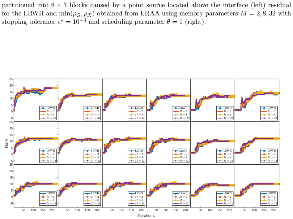
- [Throughout] There are several typos: 'paritioned' in Figure 9 caption, 'correpsonding' in §6.2.2, 'the the overall magnitude' in §6.1.1, and 'Acelleration' in the keywords. A light proofreading pass is needed.
- [§6.1.3] The description of the full-rank reference solution (“performing an explicit inverse”) is vague. Provide the precise way the reference WaveHoltz solution is computed so the error comparison is reproducible.
Circularity Check
No significant circularity: LR-WaveHoltz is a new combination with independent full-rank benchmarks, and the self-citations are to external convergence theorems.
full rationale
Walked the claimed derivation chain. The WaveHoltz fixed-point identity Π[u,iωu]^T = [u,iωu]^T is true by construction of the kernel (cos ωt − 1/4) in Eq. (5), but the paper uses this as an equivalence, not as evidence of convergence: the actual convergence claim is explicitly delegated to [8,29], which are parameter-free convergence theorems with proofs in separate publications and are not fitted to the present experiments. The low-rank step-truncation (Algorithm 3) and TT rounding (Eq. 15) are standard rank-adaptive approximations; no target quantity is defined in terms of a fitted parameter. The Anderson acceleration is inherited from [25], but its effectiveness here is demonstrated numerically against LRWH without acceleration (Figs. 5–7, 9–14), so it is not an unverified self-citation chain. The empirical checks compare against full-rank SBP references and explicit inverse solutions, so the error claims are not self-referential. The residual schedule ε_k = max{K, θhρ_k} does couple the truncation tolerance to the residual, but it does not define the claimed Helmholtz accuracy; the same experiments also report direct discrete error. The open issue that step-truncation may shift the WaveHoltz fixed point is a correctness/approximation risk, not circularity, since the paper does not claim a theorem ruling out such a shift. No step reduces to its input by construction, and no fitted parameter is renamed as a prediction.
Assumptions & free parameters
free parameters (7)
- Truncation tolerance ε (wave-solver tolerance ε̃ = ε/(2N_t)) =
ε = 1e-2 to 1e-5 h-scaled in 2D; δ = √2 ε / ||G|| in 3D
- Scheduling parameter θ =
θ = 1 in 2D, θ = 0.5 in 3D
- Floor constant K =
K = 1e-5 in 2D, K = 1e-4 in 3D
- SBP penalty parameter τ =
τ = 15
- Time-step ratio Δt/h =
0.15
- Gaussian source width δ =
δ = 1/(2ω)
- Initial and stopping tolerances ε_0, ε* =
ε* = 1e-3; ε_0 not stated for 2D
assumptions (6)
- domain assumption The SBP-SAT semidiscretization (11)–(12) is stable and satisfies an energy estimate when τ is sufficiently large.
- domain assumption The WaveHoltz filter operator Π has the stated frequency-selection property and the fixed-point iteration converges under natural assumptions.
- ad hoc to paper Step-truncation with tolerance ε does not accumulate errors large enough to break convergence of the WaveHoltz iteration.
- ad hoc to paper The WaveHoltz iterates have low SVD/TT rank at all times, with rank bounded by the rank of the truncated full-rank solution.
- standard math TT rounding in the TT-Toolbox satisfies the relative tolerance bound (15).
- domain assumption The Gaussian forcing (17) is an adequate model of a point source for the Helmholtz solutions studied.
Cite this review
Pith. "Pith review of LR-WaveHoltz: A Low-Rank Helmholtz Solver." pith.science (2026). https://pith.science/paper/LJGQPP5U
@misc{pith2026251009352,
  author       = {Pith},
  title        = {Pith review of: LR-WaveHoltz: A Low-Rank Helmholtz Solver},
  year         = {2026},
  howpublished = {\url{https://pith.science/paper/LJGQPP5U}},
  note         = {Machine review of arXiv:2510.09352}
}
read the original abstract
We propose a low-rank method for solving the Helmholtz equation. Our approach is based on the WaveHoltz method, which computes Helmholtz solutions by applying a time-domain filter to the solution of a related wave equation. The wave equation is discretized by high-order multiblock summation-by-parts finite differences. In two dimensions we seek to compress the solution in matrix form, and in three dimensions using tensor trains. To control rank growth we use step-truncation during time stepping and a low-rank Anderson acceleration for the WaveHoltz fixed point iteration. We have carried out extensive numerical experiments demonstrating the convergence and efficacy of the iterative scheme for free- and half-space problems in two and three dimensions with constant and piecewise constant wave speeds.
Figures


Figures from the paper (18 more)




Reference graph
Works this paper leans on
-
[1]
J. M. Hovem, Ray trace modeling of underwater sound propa gation. Documentation and use of the PlaneRay model, IntechOpen, 2011
2011
-
[2]
C. L. Pekeris, Theory of propagation of explosive sound i n shallow water (1948)
1948
-
[3]
F. D. Tappert, The parabolic approximation method, Wave propagation and underwater acous- tics (2005) 224–287
2005
-
[4]
O. G. Ernst, M. J. Gander, Why it is difficult to solve Helmho ltz problems with classical iterative methods, Numerical analysis of multiscale probl ems (2011) 325–363
2011
-
[5]
Y. A. Erlangga, Advances in iterative methods and precon ditioners for the Helmholtz equation, Archives of Computational Methods in Engineering 15 (2008) 37–66
2008
-
[6]
Kreiss, J
H.-O. Kreiss, J. Oliger, Comparison of accurate methods for the integration of hyperbolic equations, Tellus 24 (3) (1972) 199–215
1972
-
[7]
Hagstrom, G
T. Hagstrom, G. Hagstrom, Grid stabilization of high-or der one-sided differencing ii: Second- order wave equations, Journal of Computational Physics 231 (23) (2012) 7907–7931
2012
-
[8]
Appel¨ o, F
D. Appel¨ o, F. Garcia, O. Runborg, Waveholtz: Iterative solution of the Helmholtz equation via the wave equation, SIAM Journal on Scientific Computing 4 2 (4) (2020) A1950–A1983
2020
Show all 37 references
-
[9]
Appel¨ o, F
D. Appel¨ o, F. Garcia, A. A. Loya, O. Runborg, El-WaveHol tz: A time-domain iterative solver for time-harmonic elastic waves, Computer Methods in Appli ed Mechanics and Engineering 401 (2022) 115603
2022
-
[10]
Z. Peng, D. Appel¨ o, EM-WaveHoltz: A flexible frequency -domain method built from time- domain solvers, IEEE Transactions on Antennas and Propagat ion 70 (7) (2022) 5659–5671
2022
-
[11]
Kreiss, G
H.-O. Kreiss, G. Scherer, Finite element and finite differ ence methods for hyperbolic partial differential equations, in: Mathematical aspects of finite el ements in partial differential equa- tions, Elsevier, 1974, pp. 195–212
1974
-
[12]
M. H. Carpenter, D. Gottlieb, S. Abarbanel, Time-stabl e boundary conditions for finite- difference schemes solving hyperbolic systems: methodology and application to high-order compact schemes, Journal of Computational Physics 111 (2) ( 1994) 220–236
1994
-
[13]
Mattsson, F
K. Mattsson, F. Ham, G. Iaccarino, Stable boundary trea tment for the wave equation on second-order form, Journal of Scientific Computing 41 (2009 ) 366–383
2009
-
[14]
Mattsson, F
K. Mattsson, F. Ham, G. Iaccarino, Stable and accurate w ave-propagation in discontinuous media, Journal of Computational Physics 227 (19) (2008) 875 3–8767
2008
-
[15]
Bachmayr, Low-rank tensor methods for partial differe ntial equations, Acta Numerica 32 (2023) 1–121
M. Bachmayr, Low-rank tensor methods for partial differe ntial equations, Acta Numerica 32 (2023) 1–121
2023
-
[16]
O. Koch, C. Lubich, Dynamical low-rank approximation, SIAM Journal on Matrix Analysis and Applications 29 (2) (2007) 434–454
2007
-
[17]
Dektor, A
A. Dektor, A. Rodgers, D. Venturi, Rank-adaptive tenso r methods for high-dimensional non- linear pdes, Journal of Scientific Computing 88 (2) (2021) 36 . 28
2021
-
[18]
Appel¨ o, Y
D. Appel¨ o, Y. Cheng, Robust implicit adaptive low rank time-stepping methods for matrix differential equations, Journal of Scientific Computing 102 ( 3) (2025) 81
2025
-
[19]
I. V. Oseledets, Tensor-train decomposition, SIAM Jou rnal on Scientific Computing 33 (5) (2011) 2295–2317
2011
-
[20]
S. V. Dolgov, B. N. Khoromskij, I. V. Oseledets, Fast sol ution of parabolic problems in the ten- sor train/quantized tensor train format with initial appli cation to the Fokker–Planck equation, SIAM Journal on Scientific Computing 34 (6) (2012) A3016–A30 38
2012
-
[21]
S. V. Dolgov, A. P. Smirnov, E. Tyrtyshnikov, Low-rank a pproximation in the numerical modeling of the Farley–Buneman instability in ionospheric plasma, Journal of Computational Physics 263 (2014) 268–282
2014
-
[22]
Bebendorf, W
M. Bebendorf, W. Hackbusch, Existence of H-matrix approximants to the inverse FE-matrix of elliptic operators with l∞-coefficients, Numerische Mathematik 95 (1) (2003) 1–28
2003
-
[23]
Engquist, H
B. Engquist, H. Zhao, Approximate separability of the G reen’s function of the Helmholtz equation in the high frequency limit, Communications on Pur e and Applied Mathematics 71 (11) (2018) 2220–2274. doi:10.1002/cpa.21755
2018 doi
-
[24]
Engquist, L
B. Engquist, L. Ying, Fast directional multilevel algo rithms for oscillatory kernels, SIAM Journal on Scientific Computing 29 (4) (2007) 1710–1737
2007
-
[25]
Appel¨ o, Y
D. Appel¨ o, Y. Cheng, lrAA: Low-Rank Anderson Accelera tion, arXiv preprint arXiv:2503.03909 (2025)
2025 arXiv
-
[26]
F. B. Jensen, W. A. Kuperman, M. B. Porter, H. Schmidt, A. Tolstoy, Computational ocean acoustics, Vol. 2011, Springer, 2011
2011
-
[27]
Hagstrom, Radiation boundary conditions for the num erical simulation of waves, Acta numerica 8 (1999) 47–106
T. Hagstrom, Radiation boundary conditions for the num erical simulation of waves, Acta numerica 8 (1999) 47–106
1999
-
[28]
Appel¨ o, S
D. Appel¨ o, S. Wang, An energy-based discontinuous gal erkin method for coupled elasto- acoustic wave equations in second-order form, Internation al Journal for Numerical Methods in Engineering 119 (7) (2019) 618–638
2019
-
[30]
Y. Yang, A. Townsend, D. Appel¨ o, Anderson acceleratio n based on the h- s sobolev norm for contractive and noncontractive fixed-point operators, Jou rnal of Computational and Applied Mathematics 403 (2022) 113844
2022
-
[31]
Mattsson, J
K. Mattsson, J. Nordstr¨ om, Summation by parts operato rs for finite difference approximations of second derivatives, Journal of Computational Physics 19 9 (2) (2004) 503–540
2004
-
[32]
J. E. Hicken, D. W. Zingg, Summation-by-parts operator s and high-order quadrature, Journal of Computational and Applied Mathematics 237 (1) (2013) 111 –125
2013
-
[33]
Almquist, S
M. Almquist, S. Wang, J. Werpers, Order-preserving int erpolation for summation-by-parts operators at nonconforming grid interfaces, SIAM Journal o n Scientific Computing 41 (2) (2019) A1201–A1227. 29
2019
-
[34]
Benner, R.-C
P. Benner, R.-C. Li, N. Truhar, On the adi method for sylv ester equations, Journal of Com- putational and Applied Mathematics 233 (4) (2009) 1035–104 5
2009
-
[35]
Rotem, O
A. Rotem, O. Runborg, D. Appel¨ o, Convergence of the sem i-discrete waveholtz iteration, arXiv:2407.06929 (2024)
2024
-
[36]
Appel¨ o, J
D. Appel¨ o, J. W. Banks, W. D. Henshaw, D. W. Schwendeman , A rule of thumb for choosing points-per-wavelength for finite difference approximations of Helmholtz problems, submitted (2025)
2025
-
[37]
Sabino, Solution of large-scale Lyapunov equations via the block modified Smith method, Ph.D
J. Sabino, Solution of large-scale Lyapunov equations via the block modified Smith method, Ph.D. thesis, Rice University, Houston (2006)
2006
-
[38]
K. B. Petersen, M. S. Pedersen, et al., The matrix cookbo ok, Technical University of Denmark 7 (15) (2008) 510. A Enforcing time dependent boundary conditions In this section, we provide a short introduction to the metho d used to impose the outflow conditions in matrix form. ...
2008
Reviewed August 4, 2026 · model on record in the stance chip above.
Discussion (0). Continue with ORCID to comment.