Cost-of-capital valuation with risky assets

Filip Lindskog; Hansj\"org Albrecher; Herv\'e Zumbach

arxiv: 2511.00895 · v2 · submitted 2025-11-02 · 💱 q-fin.RM

Cost-of-capital valuation with risky assets

Hansj\"org Albrecher , Filip Lindskog , Herv\'e Zumbach This is my paper

Pith reviewed 2026-05-18 02:01 UTC · model grok-4.3

classification 💱 q-fin.RM

keywords cost-of-capital valuationbuffer capitalrisky assetslimited liabilityheavy-tailed risksinsurance liabilitiesregulatory capital

0 comments

The pith

Allowing buffer capital to be held in risky assets changes how much of the required capital comes from policyholders versus investors.

A machine-rendered reading of the paper's core claim, the machinery that carries it, and where it could break.

The paper studies cost-of-capital valuation for insurance liabilities when the buffer capital can be invested in risky assets instead of safe one-year bonds. It shows exactly how the split of that capital between policyholders and investors shifts as the riskiness of the investments rises. This matters under current regulatory rules because those rules often assume risk-free holdings, and allowing realistic investments reveals different capital burdens. The analysis uses general theory plus explicit calculations in chosen models and numerical checks to track the changes, with special attention to heavy-tailed risks where limited liability matters.

Core claim

When buffer capital is invested in risky assets such as stocks and bonds, the decomposition of this capital into contributions from policyholders and from investors varies systematically with the degree of investment risk. In the presence of heavy-tailed insurance risks, limited liability determines how much of the burden falls on each party.

What carries the argument

The decomposition of buffer capital into policyholder and investor contributions as investment risk increases

If this is right

Higher investment risk increases the portion of buffer capital borne by investors relative to policyholders.
Limited liability reduces the capital contribution required from policyholders when insurance risks have heavy tails.
Valuations of liabilities must account for the chosen investment strategy of the buffer rather than assuming risk-free holdings.
Explicit results become available in certain stochastic models that capture the varying risk levels.

Where Pith is reading between the lines

These are editorial extensions of the paper, not claims the author makes directly.

Regulators could require disclosures of buffer investment strategies when setting capital rules.
The framework could be extended to multi-period horizons where returns compound over time.
Similar decompositions might apply to other regulated sectors that hold capital buffers against uncertain liabilities.

Load-bearing premise

The effects of investing buffer capital in risky assets can be isolated and measured using general theoretical results together with specific stochastic models, without needing full details on market dynamics or correlations between assets and insurance risks.

What would settle it

Numerical results or explicit model calculations showing that the policyholder-investor split of buffer capital stays the same no matter how risky the investments become.

Figures

Figures reproduced from arXiv: 2511.00895 by Filip Lindskog, Hansj\"org Albrecher, Herv\'e Zumbach.

**Figure 2.** Figure 2: Rw 0 , Cw 0 and V w 0 for the Gaussian model with µ = 1.05, σ = 0.2, γ = 1, ρ = VaR0.005 and various values of ν corresponds to purely risk-less investment and w = 1 corresponds to purely risky investment, cf. (5)). Note that while the needed insurance premium V w 0 reduces with increasing risky asset allocation for all w, the needed solvency requirement C w 0 from shareholders increases correspondingly, … view at source ↗

**Figure 3.** Figure 3: Rw 0 , Cw 0 and V w 0 for the lognormal model with E[S1] = 1.05, E[X1] = 1, std(X) = 0.3, ρ = VaR0.005 and various values of std(S1) [PITH_FULL_IMAGE:figures/full_fig_p016_3.png] view at source ↗

**Figure 4.** Figure 4: Upper and lower bounds for V w 0 in [PITH_FULL_IMAGE:figures/full_fig_p017_4.png] view at source ↗

**Figure 5.** Figure 5: Rw 0 , Cw 0 and V w 0 for the lognormal model with E[S1] = 1.05, E[X1] = 1, std(S1) = 0.2, ρ = VaR0.005 and various values of std(X1) (a) std(X1) = 0.2 (b) std(X1) = 0.4 (c) std(X1) = 0.6 [PITH_FULL_IMAGE:figures/full_fig_p018_5.png] view at source ↗

**Figure 6.** Figure 6: Upper and lower bounds for V w 0 in [PITH_FULL_IMAGE:figures/full_fig_p018_6.png] view at source ↗

**Figure 7.** Figure 7: Rw 0 , Cw 0 and V w 0 for the lognormal model with E[S1] = 1.02, E[X1] = 1, std(X) = 0.3, ρ = VaR0.005 and various values of std(S1) (a) std(X1) = 0.2 (b) std(X1) = 0.4 (c) std(X1) = 0.6 [PITH_FULL_IMAGE:figures/full_fig_p019_7.png] view at source ↗

**Figure 8.** Figure 8: Rw 0 , Cw 0 and V w 0 for the lognormal model with E[S1] = 1.02, E[X1] = 1, std(S1) = 0.2, ρ = VaR0.005 and various values of std(X1) For example, the resulting Pareto parameters in [PITH_FULL_IMAGE:figures/full_fig_p019_8.png] view at source ↗

**Figure 9.** Figure 9: Rw 0 , Cw 0 and V w 0 for lognormal S1 and Pareto-distributed X1 with E[X1] = 1, std(X1) = 0.3, E[S1] = 1.05, ρ = VaR0.005 and various values of std(S1) (a) std(X1) = 0.2 (b) std(X1) = 0.4 (c) std(X1) = 0.6 [PITH_FULL_IMAGE:figures/full_fig_p020_9.png] view at source ↗

**Figure 10.** Figure 10: Rw 0 , Cw 0 and V w 0 for lognormal S1 and Pareto-distributed X1 with E[X1] = 1, E[S1] = 1.05, std(S1) = 0.2, ρ = VaR0.005 and various values of std(X1) Finally, it may be of interest to see the effect of the risk measure on the result. While for the normal model the expected shortfall can be replaced 20 [PITH_FULL_IMAGE:figures/full_fig_p020_10.png] view at source ↗

**Figure 11.** Figure 11: Rw 0 , Cw 0 and V w 0 for lognormal S1 and Pareto type I-distributed X1 with E[X1] = 1, E[S1] = 1.05, std(S1) = 0.2, ρ = VaR0.005 and low levels of Pareto parameter β by a value at risk with a different security level, this is not the case for the lognormal model. Figures 12 and 13 depict the analogues of Figures 3 and 5 when VaR0.005 is replaced by ES0.01 (which is the risk measure in the Swiss Solvency … view at source ↗

**Figure 12.** Figure 12: Rw 0 , Cw 0 and V w 0 for the lognormal model with E[S1] = 1.05, E[X1] = 1, std(X1) = 0.3, ρ = ES0.01 and various values of std(S1) All these numerical examples illustrate that the appropriate blending of (independent) financial risk into the management of insurance risk can drive down the necessary insurance premiums according to actuarial considerations, which may be considered as a promising insight i… view at source ↗

**Figure 13.** Figure 13: Rw 0 , Cw 0 and V w 0 for the lognormal model with E[S1] = 1.05, E[X1] = 1, std(S1) = 0.2, ρ = ES0.01 and various values of std(X1) absolute reduction of V0 through increasing w is still relatively moderate. 6 Conclusions In this paper we showed, for simple yet reasonably realistic model assumptions, that a partial investment of the solvency capital into risky assets with higher return but also higher vo… view at source ↗

read the original abstract

Cost-of-capital valuation is a well-established approach to the valuation of liabilities and is one of the cornerstones of current regulatory frameworks for the insurance industry. Standard cost-of-capital considerations typically rely on the assumption that the required buffer capital is held in risk-less one-year bonds. The aim of this work is to analyze the effects of allowing investments of the buffer capital in risky assets, e.g.~in a combination of stocks and bonds. In particular, we make precise how the decomposition of the buffer capital into contributions from policyholders and investors varies as the degree of riskiness of the investment increases, and highlight the role of limited liability in the case of heavy-tailed insurance risks. We present a combination of general theoretical results, explicit results for certain stochastic models and numerical results that emphasize the key findings.

Editorial analysis

A structured set of objections, weighed in public.

Desk editor's note, referee report, simulated authors' rebuttal, and a circularity audit. Tearing a paper down is the easy half of reading it; the pith above is the substance, this is the friction.

Desk Editor's Note private letter to a colleague

The paper extends cost-of-capital valuation by allowing risky buffer investments and tracks the resulting shift in policyholder versus investor contributions, with a focus on limited liability under heavy tails.

read the letter

The main thing to know is that this work drops the standard risk-free buffer assumption and shows how the capital split between policyholders and investors changes as the buffer is invested in riskier assets like stocks and bonds. They combine general theoretical results with explicit stochastic models and some numerical checks to make the variation with investment riskiness precise, and they point out that limited liability amplifies effects when insurance risks are heavy-tailed. That part feels like a direct response to how regulators actually think about solvency buffers today. The analysis builds cleanly on existing cost-of-capital ideas without obvious circularity or invented parameters. The models appear to isolate the riskiness effect through allocation or volatility parameters in a way that lets them compare decompositions across scenarios. One soft spot is the joint dynamics between the risky buffer assets and the insurance liabilities. The stress-test note is fair here: if the paper does not vary or report sensitivity to correlations and tail dependence, then the claimed systematic changes in decomposition could shift under different dependence structures, particularly in heavy-tailed regimes where buffer exhaustion matters most. Even moderate positive dependence might alter the split more than the riskiness parameter alone. That said, the core theoretical results still stand on their own terms if the models are internally consistent. This is for people working on insurance regulation and solvency frameworks who already know the basic cost-of-capital setup. A reader focused on practical capital rules would get value from the decomposition results and the limited-liability angle. It deserves a serious referee because the question is relevant and the approach is grounded enough to be worth tightening on the dependence assumptions.

Referee Report

2 major / 2 minor

Summary. The manuscript extends standard cost-of-capital valuation of insurance liabilities by relaxing the assumption that the required buffer capital is held exclusively in risk-free one-year bonds. It derives general theoretical results on the decomposition of buffer capital into policyholder and investor contributions, shows how this decomposition varies systematically with the degree of investment riskiness (e.g., via allocation or volatility parameters), and highlights the amplifying role of limited liability when insurance risks are heavy-tailed. The claims are supported by explicit closed-form results in selected stochastic models together with numerical illustrations.

Significance. If the decomposition results are robust, the work would be significant for regulatory frameworks such as Solvency II that rely on cost-of-capital principles. By quantifying how risky buffer investments shift the split between policyholder and investor contributions and by isolating the limited-liability effect under heavy tails, the paper supplies both a conceptual clarification and practical guidance on capital allocation. The combination of general theory, model-specific explicit solutions, and numerics is a clear strength.

major comments (2)

[§2.3] §2.3 and the model setup preceding Eq. (8): the joint dynamics (or copula) between the risky buffer-asset returns and the insurance-liability process are not specified. Because the central claim concerns the variation of the decomposition with investment riskiness and the role of limited liability under heavy tails, any unstated tail dependence would directly affect the probability of buffer exhaustion and therefore the reported split; the results need to be shown to be either independent of this choice or explicitly varied over a range of dependence parameters.
[§3] Theorem 1 (or the general decomposition result in §3): the proof appears to treat the buffer investment return as independent of the liability process. If this independence is maintained throughout, the claimed variation with riskiness may be an artifact of the independence assumption rather than a general feature; a sensitivity check or an extension to correlated cases is required to support the headline conclusion.

minor comments (2)

[Figure 4] Figure 4 (or the numerical panel showing heavy-tailed cases): the x-axis label for investment riskiness should explicitly state whether it is volatility, equity allocation weight, or another parameter; without this the reader cannot map the plotted curves to the theoretical statements.
[§2.1] Notation: the symbol for the cost-of-capital rate is introduced in two places with slightly different subscripts; a single consistent definition in §2.1 would improve readability.

Simulated Author's Rebuttal

2 responses · 0 unresolved

We thank the referee for the careful and constructive review. The comments highlight an important aspect of model robustness that we will address in the revision. Below we respond point by point to the major comments.

read point-by-point responses

Referee: [§2.3] §2.3 and the model setup preceding Eq. (8): the joint dynamics (or copula) between the risky buffer-asset returns and the insurance-liability process are not specified. Because the central claim concerns the variation of the decomposition with investment riskiness and the role of limited liability under heavy tails, any unstated tail dependence would directly affect the probability of buffer exhaustion and therefore the reported split; the results need to be shown to be either independent of this choice or explicitly varied over a range of dependence parameters.

Authors: We agree that the joint distribution is not fully specified beyond the independence assumption used throughout the paper. This assumption is stated in the model setup preceding Eq. (8) and is maintained to obtain the closed-form results in the selected stochastic models. We acknowledge that unmodeled tail dependence could alter the probability of buffer exhaustion and thus the reported decomposition, particularly for heavy-tailed risks. In the revised manuscript we will add a dedicated subsection (new §2.4) that discusses this limitation and provides numerical illustrations under alternative dependence structures. Specifically, we will report results for Gaussian and Clayton copulas with correlation parameters ranging from 0 to 0.8, demonstrating that the qualitative patterns—namely the shift in contributions with increasing investment riskiness and the amplifying effect of limited liability—remain directionally unchanged under moderate dependence. revision: yes
Referee: [§3] Theorem 1 (or the general decomposition result in §3): the proof appears to treat the buffer investment return as independent of the liability process. If this independence is maintained throughout, the claimed variation with riskiness may be an artifact of the independence assumption rather than a general feature; a sensitivity check or an extension to correlated cases is required to support the headline conclusion.

Authors: The proof of Theorem 1 does rely on independence between the buffer investment return and the liability process; this is used to factor the relevant expectations and obtain the explicit decomposition formula. While the theoretical variation with riskiness is therefore derived under independence, the mechanism (increased volatility of the buffer raising the likelihood of exhaustion and thereby reallocating contributions) is economically intuitive. To support the headline conclusion beyond the independence case, the revision will include a new numerical sensitivity study in §4. We will simulate paths with nonzero correlation between asset returns and liabilities and show that the monotonicity of the policyholder/investor split with respect to the investment-risk parameter persists for correlation values up to 0.5. We note that a fully general proof without any independence assumption would require substantially different techniques and is left for future work. revision: partial

Circularity Check

0 steps flagged

No significant circularity; derivation is model-driven and self-contained

full rationale

The paper derives the decomposition of buffer capital contributions via general theoretical results combined with explicit stochastic models and numerical illustrations. No steps reduce by construction to fitted parameters renamed as predictions, self-definitional loops, or load-bearing self-citations whose validity depends on the current work. The variation with investment riskiness follows directly from the chosen risk processes and limited-liability mechanics rather than being imposed by ansatz or renaming of known patterns. The analysis remains independent of any unverified uniqueness theorems imported from the authors' prior work.

Axiom & Free-Parameter Ledger

0 free parameters · 0 axioms · 0 invented entities

Based solely on the abstract, the central claim rests on standard insurance valuation assumptions that are relaxed here; no explicit free parameters, new axioms, or invented entities are identifiable without the full text.

pith-pipeline@v0.9.0 · 5665 in / 1140 out tokens · 33023 ms · 2026-05-18T02:01:14.646177+00:00 · methodology

discussion (0)

Lean theorems connected to this paper

Citations machine-checked in the Pith Canon. Every link opens the source theorem in the public Lean library.

IndisputableMonolith/Cost/FunctionalEquation.lean washburn_uniqueness_aczel unclear

?

unclear
Relation between the paper passage and the cited Recognition theorem.

V_0 = 1/(1+η) E[(R_0 Z_1) ∧ X_1] + η/(1+η) R_0 + 1/(1+η) R_0 E[1-Z_1]; R_0 solves ρ(R_0 Z_1 - X_1)=0 with ρ=VaR_α or ES_α
IndisputableMonolith/Foundation/BranchSelection.lean branch_selection unclear

?

unclear
Relation between the paper passage and the cited Recognition theorem.

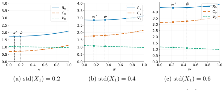
Proposition 2.4: under S_1 ≥_icx 1 and 1+η ≥ μ_w, w ↦ V_w_0 decreasing for small w

What do these tags mean?

matches: The paper's claim is directly supported by a theorem in the formal canon.
supports: The theorem supports part of the paper's argument, but the paper may add assumptions or extra steps.
extends: The paper goes beyond the formal theorem; the theorem is a base layer rather than the whole result.
uses: The paper appears to rely on the theorem as machinery.
contradicts: The paper's claim conflicts with a theorem or certificate in the canon.
unclear: Pith found a possible connection, but the passage is too broad, indirect, or ambiguous to say the theorem truly supports the claim.

Reference graph

Works this paper leans on

25 extracted references · 25 canonical work pages

[1]

Albrecher and M

H. Albrecher and M. Dacorogna. Allocating capital to time: Intro- ducing credit migration for measuring time-related risks.Scandinavian Actuarial Journal, 2025, to appear

work page 2025
[2]

Albrecher, K.-T

H. Albrecher, K.-T. Eisele, M. Steffensen, and M. V. W¨ uthrich. On the cost-of-capital rate under incomplete market valuation.Journal of Risk and Insurance, 89(4):1139–1158, 2022

work page 2022
[3]

Artzner, K.-T

P. Artzner, K.-T. Eisele, and T. Schmidt. Insurance-finance arbitrage. Mathematical Finance, 34:739–773, 2024

work page 2024
[4]

Barigou, V

K. Barigou, V. Bignozzi, and A. Tsanakas. Insurance valuation: A two- step generalised regression approach.ASTIN Bulletin, 52(1):211–245, 2022

work page 2022
[5]

Barigou and J

K. Barigou and J. Dhaene. Fair valuation of insurance liabilities via mean-variance hedging in a multi-period setting.Scandinavian Actu- arial Journal, 2019(2):163–187, 2019

work page 2019
[6]

Delong, J

L. Delong, J. Dhaene, and K. Barigou. Fair valuation of insurance lia- bility cash-flow streams in continuous time: Theory.Insurance: Math- ematics and Economics, 88:196–208, 2019. 28

work page 2019
[7]

Denuit, J

M. Denuit, J. Dhaene, M. Goovaerts, and R. Kaas.Actuarial theory for dependent risks: measures, orders and models. John Wiley & Sons, 2006

work page 2006
[8]

Dhaene, B

J. Dhaene, B. Stassen, K. Barigou, D. Linders, and Z. Chen. Fair valu- ation of insurance liabilities: Merging actuarial judgement and market- consistency.Insurance: Mathematics and Economics, 76:14–27, 2017

work page 2017
[9]

Engler and F

N. Engler and F. Lindskog. Approximations of multi-period liability values by simple formulas.Insurance: Mathematics and Economics, 123:103112, 2025

work page 2025
[10]

Engsner, M

H. Engsner, M. Lindholm, and F. Lindskog. Insurance valuation: A computable multi-period cost-of-capital approach.Insurance: Mathe- matics and Economics, 72:250–264, 2017

work page 2017
[11]

Engsner, F

H. Engsner, F. Lindskog, and J. Thøgersen. Multiple-prior valuation of cash flows subject to capital requirements.Insurance: Mathematics and Economics, 111:41–56, 2023

work page 2023
[12]

Directive 2009/138/EC (Solvency II).Official Journal of European Union, 335, 2009

European Union. Directive 2009/138/EC (Solvency II).Official Journal of European Union, 335, 2009

work page 2009
[13]

Commission delegated regulation (EU) 2015/35.Of- ficial Journal of the European Union, 12, 2015

European Union. Commission delegated regulation (EU) 2015/35.Of- ficial Journal of the European Union, 12, 2015

work page 2015
[14]

Directive 2025/2 amending Directive 2009/138/EC

European Union. Directive 2025/2 amending Directive 2009/138/EC. Official Journal of the European Union, 2, 2025

work page 2025
[15]

Technical document on the Swiss Solvency Test

Federal Office of Private Insurance. Technical document on the Swiss Solvency Test. Technical report, Federal Office of Private Insurance, Switzerland, 2006

work page 2006
[16]

Filipovi´ c, R

D. Filipovi´ c, R. Kremslehner, and A. Muermann. Optimal investment and premium policies under risk shifting and solvency regulation.Jour- nal of Risk and Insurance, 82(2):261–288, 2015

work page 2015
[17]

Floreani

A. Floreani. Risk margin estimation through the cost of capital ap- proach: Some conceptual issues.The Geneva Papers on Risk and In- surance: Issues and Practice, 36:226–253, 2011

work page 2011
[18]

F¨ ollmer and A

H. F¨ ollmer and A. Schied.Stochastic finance. An introduction in dis- crete time.De Gruyter Textb. Berlin: de Gruyter, 4th revised edition edition, 2016

work page 2016
[19]

H. Jones. EU agrees to ease capital rules for insurers to boost in- vestment. Available at https://www.reuters.com/business/finance/eu- agrees-ease-capital-rules-insurers-boost-investment-2023-12-13/, 2023. 29

work page 2023
[20]

Koch-Medina and C

P. Koch-Medina and C. Munari.Market-Consistent Prices. Springer, Heidelberg, 2020

work page 2020
[21]

S. J. Mildenhall and J. A. Major.Pricing Insurance Risk: Theory and practice. John Wiley & Sons, 2022

work page 2022
[22]

C. M¨ ohr. Market-consistent valuation of insurance liabilities by cost of capital.ASTIN Bulletin, 41(2):315–341, 2011

work page 2011
[23]

Oberpriller, M

K. Oberpriller, M. Ritter, and T. Schmidt. Robust asymptotic insurance-finance arbitrage.European Actuarial Journal, 14(3):929– 963, 2024

work page 2024
[24]

Salahnejhad Ghalehjooghi and A

A. Salahnejhad Ghalehjooghi and A. Pelsser. A market-and time- consistent extension for the EIOPA risk margin.European Actuarial Journal, 13(2):517–539, 2023

work page 2023
[25]

Salzmann and M

R. Salzmann and M. V. W¨ uthrich. Cost-of-capital margin for a general insurance liability runoff.ASTIN Bulletin, 40(2):415–451, 2010. 30

work page 2010

[1] [1]

Albrecher and M

H. Albrecher and M. Dacorogna. Allocating capital to time: Intro- ducing credit migration for measuring time-related risks.Scandinavian Actuarial Journal, 2025, to appear

work page 2025

[2] [2]

Albrecher, K.-T

H. Albrecher, K.-T. Eisele, M. Steffensen, and M. V. W¨ uthrich. On the cost-of-capital rate under incomplete market valuation.Journal of Risk and Insurance, 89(4):1139–1158, 2022

work page 2022

[3] [3]

Artzner, K.-T

P. Artzner, K.-T. Eisele, and T. Schmidt. Insurance-finance arbitrage. Mathematical Finance, 34:739–773, 2024

work page 2024

[4] [4]

Barigou, V

K. Barigou, V. Bignozzi, and A. Tsanakas. Insurance valuation: A two- step generalised regression approach.ASTIN Bulletin, 52(1):211–245, 2022

work page 2022

[5] [5]

Barigou and J

K. Barigou and J. Dhaene. Fair valuation of insurance liabilities via mean-variance hedging in a multi-period setting.Scandinavian Actu- arial Journal, 2019(2):163–187, 2019

work page 2019

[6] [6]

Delong, J

L. Delong, J. Dhaene, and K. Barigou. Fair valuation of insurance lia- bility cash-flow streams in continuous time: Theory.Insurance: Math- ematics and Economics, 88:196–208, 2019. 28

work page 2019

[7] [7]

Denuit, J

M. Denuit, J. Dhaene, M. Goovaerts, and R. Kaas.Actuarial theory for dependent risks: measures, orders and models. John Wiley & Sons, 2006

work page 2006

[8] [8]

Dhaene, B

J. Dhaene, B. Stassen, K. Barigou, D. Linders, and Z. Chen. Fair valu- ation of insurance liabilities: Merging actuarial judgement and market- consistency.Insurance: Mathematics and Economics, 76:14–27, 2017

work page 2017

[9] [9]

Engler and F

N. Engler and F. Lindskog. Approximations of multi-period liability values by simple formulas.Insurance: Mathematics and Economics, 123:103112, 2025

work page 2025

[10] [10]

Engsner, M

H. Engsner, M. Lindholm, and F. Lindskog. Insurance valuation: A computable multi-period cost-of-capital approach.Insurance: Mathe- matics and Economics, 72:250–264, 2017

work page 2017

[11] [11]

Engsner, F

H. Engsner, F. Lindskog, and J. Thøgersen. Multiple-prior valuation of cash flows subject to capital requirements.Insurance: Mathematics and Economics, 111:41–56, 2023

work page 2023

[12] [12]

Directive 2009/138/EC (Solvency II).Official Journal of European Union, 335, 2009

European Union. Directive 2009/138/EC (Solvency II).Official Journal of European Union, 335, 2009

work page 2009

[13] [13]

Commission delegated regulation (EU) 2015/35.Of- ficial Journal of the European Union, 12, 2015

European Union. Commission delegated regulation (EU) 2015/35.Of- ficial Journal of the European Union, 12, 2015

work page 2015

[14] [14]

Directive 2025/2 amending Directive 2009/138/EC

European Union. Directive 2025/2 amending Directive 2009/138/EC. Official Journal of the European Union, 2, 2025

work page 2025

[15] [15]

Technical document on the Swiss Solvency Test

Federal Office of Private Insurance. Technical document on the Swiss Solvency Test. Technical report, Federal Office of Private Insurance, Switzerland, 2006

work page 2006

[16] [16]

Filipovi´ c, R

D. Filipovi´ c, R. Kremslehner, and A. Muermann. Optimal investment and premium policies under risk shifting and solvency regulation.Jour- nal of Risk and Insurance, 82(2):261–288, 2015

work page 2015

[17] [17]

Floreani

A. Floreani. Risk margin estimation through the cost of capital ap- proach: Some conceptual issues.The Geneva Papers on Risk and In- surance: Issues and Practice, 36:226–253, 2011

work page 2011

[18] [18]

F¨ ollmer and A

H. F¨ ollmer and A. Schied.Stochastic finance. An introduction in dis- crete time.De Gruyter Textb. Berlin: de Gruyter, 4th revised edition edition, 2016

work page 2016

[19] [19]

H. Jones. EU agrees to ease capital rules for insurers to boost in- vestment. Available at https://www.reuters.com/business/finance/eu- agrees-ease-capital-rules-insurers-boost-investment-2023-12-13/, 2023. 29

work page 2023

[20] [20]

Koch-Medina and C

P. Koch-Medina and C. Munari.Market-Consistent Prices. Springer, Heidelberg, 2020

work page 2020

[21] [21]

S. J. Mildenhall and J. A. Major.Pricing Insurance Risk: Theory and practice. John Wiley & Sons, 2022

work page 2022

[22] [22]

C. M¨ ohr. Market-consistent valuation of insurance liabilities by cost of capital.ASTIN Bulletin, 41(2):315–341, 2011

work page 2011

[23] [23]

Oberpriller, M

K. Oberpriller, M. Ritter, and T. Schmidt. Robust asymptotic insurance-finance arbitrage.European Actuarial Journal, 14(3):929– 963, 2024

work page 2024

[24] [24]

Salahnejhad Ghalehjooghi and A

A. Salahnejhad Ghalehjooghi and A. Pelsser. A market-and time- consistent extension for the EIOPA risk margin.European Actuarial Journal, 13(2):517–539, 2023

work page 2023

[25] [25]

Salzmann and M

R. Salzmann and M. V. W¨ uthrich. Cost-of-capital margin for a general insurance liability runoff.ASTIN Bulletin, 40(2):415–451, 2010. 30

work page 2010