REVIEW 3 major objections 6 minor 68 references
Sparse Source Identification in Transient Advection-Diffusion Problems with a Primal-Dual-Active-Point Strategy
T0 review · 3 major / 6 minor · reviewed 2026-08-04 · deepseek-v4-flash
Pith's one-line read A convex sparse-optimization reformulation turns contaminant source identification into a tractable problem whose minimizers are finitely many point sources, and a primal-dual-active-point algorithm finds them with only a handful of forward
desk verdict Solid engineering adaptation of PDAP/Radon-norm sparse inversion to contaminant source identification; the numerics are broad and plausible, but the reported accuracy is not covered by the convergence theory because of a heuristic cluster-merging post-processing step. read the letter →
The pith
A machine-rendered reading of the paper's core claim, the machinery that carries it, and where it could break.
The reading
What carries the argument
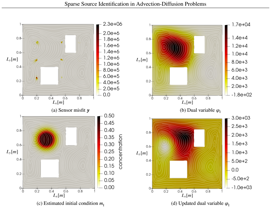
The load-bearing object is the Radon-norm-regularized objective over the cone of positive measures, and the identity that makes it algorithmic is the pre-dual relation y^T F(mu) = ∫ phi^I d mu^I + ∫ phi^C d mu^C, where (phi^I, phi^C) = -F* y is the solution of the adjoint advection-diffusion problem with reversed wind. This identity converts the infinite-dimensional optimality condition into a finite certificate: a candidate measure is optimal iff the convolved adjoint fields stay below alpha everywhere and touch alpha at every support point. The Primal-Dual-Active-Point (PDAP) algorithm exploits the certificate by greedily inserting the global maximizer of the dual field, then solving a con
What would settle it
Generate synthetic sensor data with the two-building benchmark using the true wind field, then run Algorithm 1 with a wind field perturbed by a 10% rotation or with a time-varying wind during the observation window; if the reconstructed source center moves by more than the benchmark's ~0.001 m error, the known-wind assumption is the load-bearing limitation.
Extended reading notes
Core claim
The paper's central claim is that the conventionally hard, nonconvex problem of finding an unknown number of point-like contaminant sources can be relaxed without loss: model the source as a positive Radon measure mu and minimize J(mu)=1/(2σ^2)||F(mu)-d||^2 + alpha(mu_I(Ω)+mu_C(Ω)). Theorem 1 states that this convex problem has a minimizer supported on at most N_obs points, so the relaxed solution is exactly sparse, and a pair (mu_I, mu_C) is optimal precisely when the dual variables phi^I, phi^C (adjoint fields convolved with source shape functions) never exceed alpha and equal alpha on the support. Algorithm 1 realizes that characterization: compute the misfit, solve one adjoint problem to
Load-bearing premise
The whole pipeline assumes the wind vector field is known, fixed, smooth, bounded, and divergence-free, so if the actual wind differs or changes over the measurement window, the adjoint-based candidate locations and final source estimates are unreliable.
Editorial extensions
If this is right
- The relaxation is exact in the sense that at least one optimal reconstruction is a sum of finitely many Dirac delta sources, so sparsity is a theorem, not a heuristic.
- Because the number of atoms never exceeds the number of observations, the method can in principle identify multiple distinct release points from few sensors; the two-source benchmark shows separation where L2 regularization yields a single smooth lump.
- Computational cost scales mildly with data: each iteration requires at most two forward and one adjoint PDE solve, and in the reported tests adding sensors reduces the number of iterations.
- The same framework handles initial-condition releases (instantaneous) and continuous source terms, with source shapes ranging from point Diracs to elliptic-PDE-defined profiles.
- In the large plant-site test, all eight sources were located with a maximum error below 11 m on a roughly 500 m square domain using 27 iterations, suggesting practical emergency-response feasibility.
Reading between the lines
- If the wind field is uncertain, the dual field—and hence every candidate insertion—is computed under the wrong transport direction; a natural extension the paper does not develop is to make the wind an unknown or to average over an ensemble of wind fields, which would test how strongly the method depends on this input.
- The discretization to mesh nodes induces clustering of near-optimal sources around true off-grid locations; the paper's heuristic barycentric merge is a post-process, not part of the optimization, so a sliding/refinement variant could remove this artifact and sharpen location estimates.
- The method's reliance on only forward/adjoint solves and its insensitivity to added sensors suggest it could transfer to other linear wave-type inverse problems, such as acoustic or seismic source localization, where the same convex measure-lifting arguments apply.
- Because the objective is convex and the certificate is explicit, the dual variables also give a principled criterion for placing new sensors: insert them where the dual field is still near its upper bound, connecting this work to optimal experimental design.
Editorial analysis
A structured set of objections, weighed in public.
Referee Report
Summary. The manuscript develops a variational regularization approach for identifying sparse contaminant sources in transient linear advection-diffusion equations from pointwise-in-time concentration measurements. The unknown source is represented as a positive Radon measure; the objective combines a quadratic data misfit with a Radon-norm/total-variation penalty. Theorem 1 states existence of sparse minimizers and a dual optimality condition; Corollary 1 gives an intensity subproblem. Algorithm 1 is a PDAP strategy that alternates between inserting locations where the dual variable exceeds α and re-optimizing intensities, with a claimed O(1/k) objective convergence in the continuum setting. Section 4 discretizes the forward/adjoint PDEs with stabilized finite elements and restricts source measures to grid-node Diracs, adding a heuristic barycentric cluster-merging step. Numerical experiments on 2D/3D benchmark geometries and two realistic domains compare favorably with an L2-regularized approach in accuracy and PDE-solve counts.
Significance. The paper addresses a practically important problem and contains useful theory: the convex relaxation is clean, Theorem 1 and Corollary 1 provide a solid foundation, and the numerical evidence suggests that PDAP can work on realistic geometries with few PDE solves. If the discretization/post-processing gap is closed, the method would be a valuable addition. At present, however, the quantitative claims are not fully supported: the analyzed algorithm is the continuum PDAP, while the implemented algorithm restricts candidates to grid nodes and relies on an unanalyzed post-processing step; the numerical validation is synthetic and uses the same source generators for ground truth and inversion, with per-case tuned α. These issues are fixable but require additional analysis or experiments.
major comments (3)
- [§4 (after Eq. (18))] The implementation replaces M_+(Ω) by the cone of node Diracs and replaces Step 3's global maximization by a search over finite-element nodes. The convergence statements in Section 3—including the finite-termination bound (13)—are for the continuum PDAP with exact global maximizers and exact subproblem solves. No theorem links the grid-restricted minimizers to minimizers of (P) as h→0, and Remark 2 establishes exactness of the node maximum only for piecewise-linear elements with φ3=δ; the experiments in §§5.1, 5.3.1, 5.3.2 and 5.3.4 use φ1 or φ2. The clustering caused by off-grid sources is repaired with a heuristic barycentric merge, and Tables 1 and 3 report the post-processed locations. The reported accuracy is therefore not a consequence of the PDAP theory; it can depend on the merging heuristic. Please provide a mesh-refinement study of the reconstructed source and either an error a
- [§3, Algorithm 1 Step 5 / §4] Because candidate insertion is based on the maximum over the node set, the algorithm can stop even when the continuous dual maximum exceeds α+tol in an element interior. For φ1 and φ2 the dual φ^k is not piecewise-linear or is not represented in the finite-element space, so such interior maxima can be missed; this invalidates the stopping certificate and the bound (13) for the implemented method. A local refinement or quadrature check of the maximum, or a proof that the discrete maximum suffices for the relevant generators, is required.
- [§5, Tables 1–3] The numerical validation is self-referential in two respects: all ground truths are generated from the same shape functions φ1, φ2, φ3 that are used in the inversion, and α is selected per test case (e.g., 'based on empirical evaluation' in §5.4). The claimed superiority over L2-regularization is therefore demonstrated only in an idealized setting. Please include model-mismatch experiments (e.g., reconstruct a φ1 source with the φ2 generator, or a source whose shape is not in the dictionary), a sensitivity analysis or systematic rule for choosing α, and multiple noise realizations or error bars.
minor comments (6)
- [§5.3.1, Table 2] In the five-sensor case (cases c/d), the L2 method has 16 online PDE solves versus PDAP's 20; the statement that PDAP 'clearly outperforms' is based on total online+offline cost. Please state the comparison metric explicitly and also discuss the online-only view, which is relevant for real-time deployment.
- [§5.2] Typo: 'PDAD algorithm' should be 'PDAP algorithm'.
- [§2.1] The known, divergence-free wind field assumption is stated but not discussed as a limitation for emergency-response applications. A brief paragraph on sensitivity to wind-field errors would help contextualize the numerical results.
- [§5.4] The clustering radius of 40 m is an additional free parameter; its influence on the quantitative results in Table 3 should be reported.
- [§3, Eq. (13)] The convergence rate and finite-termination bound are adapted from prior work without proof. A short proof sketch or a precise statement of the assumptions needed for Eq. (13) in this setting would make the paper more self-contained.
- [§5, Figure 7] The mesh-independence study is performed only for the forward/adjoint discretization, not for the reconstructed source locations. A companion study for the inverse reconstructions would directly address the discretization gap noted in the major comments.
Circularity Check
No significant circularity: the inversion is data-driven and the cited convergence theory is prior independent work rather than a restatement of the paper's inputs.
full rationale
The core derivation is not circular. The source estimate is obtained by minimizing the convex objective (P) over positive Radon measures; the location variables appear only through the misfit term and the Radon penalty, and their optimality is characterized by the dual support condition (7). Theorem 1's sparse-minimizer existence is proved via the external convex representer theorem [41,42] and extremal-point arguments from [43], not by assuming the conclusion. The PDAP convergence statements are adapted from [34] and [48,49]; although D. Walter is an author of those works, they are prior, independently stated mathematical results whose assumptions do not include the numerical outputs of this paper, so invoking them is legitimate support rather than a self-citation chain forcing the result. The heuristic cluster-merging post-processing, hand-tuned alpha, and the gap between continuous global maximization and grid-node search are real limitations and correctness risks, but they are not circular reductions: the post-processed source location is still determined from the measured data through the optimization, and no fitted ground-truth value is renamed as a prediction. The synthetic benchmarks reuse the same shape functions as the inversion, which is a manufactured-data validation choice, not an equivalence between inputs and outputs at the derivation level. Accordingly, no step in the claimed derivation is identical to its input by construction.
Assumptions & free parameters
free parameters (3)
- Regularization parameter α =
200–1500 per test case
- Post-processing clustering radius =
40 m (chemistry plant case)
- Source shape parameters =
r=0.26/0.25/10 m; η=1, γ=100
assumptions (6)
- domain assumption Known, smooth, bounded, divergence-free wind vector field v
- domain assumption Source is a positive superposition of finitely many atoms with known shape functions φ_I and φ_C
- domain assumption Measurement model: point evaluations plus Gaussian white noise with known variance σ²
- standard math Existence/regularity of a unique weak solution to the forward advection-diffusion equation
- standard math Convex representer theorem gives sparse minimizers with N_I + N_C ≤ N_obs
- standard math PDAP convergence O(1/k) and finite termination
Cite this review
Pith. "Pith review of Sparse Source Identification in Transient Advection-Diffusion Problems with a Primal-Dual-Active-Point Strategy." pith.science (2026). https://pith.science/paper/XYVCHV3S
@misc{pith2026251102552,
  author       = {Pith},
  title        = {Pith review of: Sparse Source Identification in Transient Advection-Diffusion Problems with a Primal-Dual-Active-Point Strategy},
  year         = {2026},
  howpublished = {\url{https://pith.science/paper/XYVCHV3S}},
  note         = {Machine review of arXiv:2511.02552}
}
abstract
This work presents a mathematical model to enable rapid prediction of airborne contaminant transport based on scarce sensor measurements. The method is designed for applications in critical infrastructure protection (CIP), such as evacuation planning following contaminant release. In such scenarios, timely and reliable decision-making is essential, despite limited observation data. To identify contaminant sources, we formulate an inverse problem governed by an advection-diffusion equation. Given the problem's underdetermined nature, we further employ a variational regularization ansatz and model the unknown contaminant sources as distribution over the spatial domain. To efficiently solve the arising inverse problem, we employ a problem-specific variant of the Primal-Dual-Active-Point (PDAP) algorithm which efficiently approximates sparse minimizers of the inverse problem by alternating between greedy location updates and source intensity optimization. The approach is demonstrated on two- and three-dimensional test cases involving both instantaneous and continuous contaminant sources and outperforms state-of-the-art techniques with $L^2$-regularization. Its effectiveness is further illustrated in complex domains with real-world building geometries imported from OpenStreetMap.
Figures


Figures from the paper (15 more)




Reference graph
Works this paper leans on
-
[1]
J. Boris, The threat of chemical and biological terrorism: preparing a response, Computing in Science & Engi- neering 4 (2) (2002) 22–32.doi:10.1109/5992.988644
arXiv 2002
-
[2]
G. Patnaik, J. P. Boris, F. F. Grinstein, J. P. Iselin, D. Hertwig, Large scale urban simulations with fct, in: D. Kuzmin, R. Löhner, S. Turek (Eds.), Flux-Corrected Transport, Scientific Computation, Springer Netherlands, Dordrecht, 2012, pp. 91–117.doi:10.1007/978-94-007-4038-9_4
-
[3]
M. von Danwitz, J. Bonari, P. Franz, L. Kühn, M. Mattuschka, A. Popp, Contaminant dispersion simulation in a digital twin framework for critical infrastructure protection.doi:10.23967/eccomas.2024.301
-
[4]
N. S. Holmes, L. Morawska, A review of dispersion modelling and its application to the dispersion of particles: An overview of different dispersion models available, Atmospheric Environment 40 (30) (2006) 5902–5928. doi:10.1016/j.atmosenv.2006.06.003
-
[5]
M. Hutchinson, H. Oh, W.-H. Chen, A review of source term estimation methods for atmospheric dispersion events using static or mobile sensors, Information Fusion 36 (2017) 130–148.doi:10.1016/j.inffus.2016. 11.010
-
[6]
R. Khodayi-mehr, W. Aquino, M. M. Zavlanos, Model-based active source identification in complex environ- ments, IEEE Transactions on Robotics 35 (3) (2019) 633–652.doi:10.1109/TRO.2019.2894039. 21 Sparse Source Identification in Advection-Diffusion Problems
arXiv 2019
-
[9]
T. Wiedemann, P. Hinsen, V . P. Ruiz, D. Shutin, A. J. Lilienthal, Domain knowledge assisted gas tomography, in: 2024 IEEE International Symposium on Olfaction and Electronic Nose (ISOEN), IEEE, 2024, pp. 1–3. doi:10.1109/ISOEN61239.2024.10556226
arXiv 2024
-
[10]
N. Arystanbekova, Application of gaussian plume models for air pollution simulation at instantaneous emissions, Mathematics and Computers in Simulation 67 (4-5) (2004) 451–458.doi:10.1016/j.matcom.2004.06.023
Show all 68 references
-
[11]
Ulfah, S
S. Ulfah, S. A. Awalludin, Wahidin, Advection-diffusion model for the simulation of air pollution distribu- tion from a point source emission, Journal of Physics: Conference Series 948 (2018) 012067.doi:10.1088/ 1742-6596/948/1/012067
2018
-
[12]
Maronga, S
B. Maronga, S. Banzhaf, C. Burmeister, T. Esch, R. Forkel, D. Fröhlich, V . Fuka, K. F. Gehrke, J. Geleti ˇc, S. Giersch, T. Gronemeier, G. Groß, W. e. a. Heldens, Overview of the palm model system 6.0, Geoscientific Model Development 13 (3) (2020) 1335–1372.doi:10.5194/gmd-13...
2020 doi
-
[13]
von Danwitz, V
M. von Danwitz, V . Karyofylli, N. Hosters, M. Behr, Simplex space–time meshes in compressible flow simula- tions, International Journal for Numerical Methods in Fluids 91 (1) (2019) 29–48.doi:10.1002/fld.4743
2019 doi
-
[14]
Towers, B
P. Towers, B. L. Jones, Real-time wind field reconstruction from lidar measurements using a dynamic wind model and state estimation, Wind Energy 19 (1) (2016) 133–150.doi:10.1002/we.1824
2016 doi
-
[15]
Y . Chen, D. Wang, D. Feng, G. Tian, V . Gupta, R. Cao, M. Wan, S. Chen, Three-dimensional spatiotemporal wind field reconstruction based on lidar and multi-scale pinn, Applied Energy 377 (2025) 124577.doi:10. 1016/j.apenergy.2024.124577
2025
-
[16]
R. A. S. Albani, V . V . L. Albani, H. S. Migon, A. J. Silva Neto, Uncertainty quantification and atmospheric source estimation with a discrepancy-based and a state-dependent adaptative mcmc, Environmental Pollution 290 (2021) 118039.doi:10.1016/j.envpol.2021.118039
2021
-
[17]
S. M. Gorelick, B. Evans, I. Remson, Identifying sources of groundwater pollution: An optimization approach, Water Resources Research 19 (3) (1983) 779–790.doi:10.1029/WR019i003p00779
1983 doi
-
[18]
R. Tsai, S. Osher, Y . Li, Heat source identification based on𝑙 1 constrained minimization, Inverse Problems and Imaging 8 (1) (2014) 199–221.doi:10.3934/ipi.2014.8.199
2014 doi
-
[19]
Villa, N
U. Villa, N. Petra, O. Ghattas, hippylib, ACM Transactions on Mathematical Software 47 (2) (2021) 1–34. doi:10.1145/3428447
2021 doi
-
[20]
Petra, G
N. Petra, G. Stadler, Model variational inverse problems governed by partial differential equations,https: //math.nyu.edu/~stadler/papers/PetraStadler11.pdf
-
[21]
F. Key, M. von Danwitz, F. Ballarin, G. Rozza, Model order reduction for deforming domain problems in a time– continuous space–time setting, International Journal for Numerical Methods in Engineering 124 (23) (2023) 5125–5150.doi:10.1002/nme.7342
2023 doi
-
[22]
Dinkel, C
M. Dinkel, C. M. Geitner, G. Robalo Rei, J. Nitzler, W. A. Wall, Solving bayesian inverse problems with ex- pensive likelihoods using constrained gaussian processes and active learning, Inverse Problems 40 (9) (2024) 095008.doi:10.1088/1361-6420/ad5eb4
2024 doi
-
[23]
A. M. Stuart, Inverse problems: A bayesian perspective, Acta Numerica 19 (2010) 451–559.doi:10.1017/ S0962492910000061
2010
-
[24]
Nitzler, J
J. Nitzler, J. Biehler, N. Fehn, P.-S. Koutsourelakis, W. A. Wall, A generalized probabilistic learning approach for multi-fidelity uncertainty quantification in complex physical simulations, Computer Methods in Applied Me- chanics and Engineering 400 (2022) 115600.doi:10.1016...
2022
-
[25]
Bredies, H
K. Bredies, H. K. Pikkarainen, Inverse problems in spaces of measures, ESAIM, Control Optim. Calc. Var. 19 (1) (2013) 190–218.doi:10.1051/cocv/2011205
2013
-
[26]
Scherzer, B
O. Scherzer, B. Walch, Sparsity regularization for radon measures, in: X.-C. Tai, K. Mørken, M. Lysaker, K.- A. Lie (Eds.), Scale Space and Variational Methods in Computer Vision, Springer Berlin Heidelberg, Berlin, Heidelberg, 2009, pp. 452–463.doi:10.1007/978-3-642-02256-2_38
2009 doi
-
[27]
Huynh, K
P.-T. Huynh, K. Pieper, D. Walter, Towards optimal sensor placement for inverse problems in spaces of measures, Inverse Problems 40 (5) (2024) 055007.doi:10.1088/1361-6420/ad2cf8. 22 Sparse Source Identification in Advection-Diffusion Problems
2024 doi
-
[28]
Casas, K
E. Casas, K. Kunisch, Using sparse control methods to identify sources in linear diffusion-convection equations, Inverse Problems 35 (11) (2019) 114002.doi:10.1088/1361-6420/ab331c
2019 doi
-
[29]
Leykekhman, B
D. Leykekhman, B. Vexler, D. Walter, Numerical analysis of sparse initial data identification for parabolic prob- lems, ESAIM: Mathematical Modelling and Numerical Analysis 54 (4) (2020) 1139–1180.doi:10.1051/ m2an/2019083
2020
-
[30]
Biccari, Y
U. Biccari, Y . Song, X. Yuan, E. Zuazua, A two-stage numerical approach for the sparse initial source identifi- cation of a diffusion–advection equation, Inverse Problems 39 (9) (2023) 095003.doi:10.1088/1361-6420/ ace548
2023 doi
-
[31]
Monge, E
A. Monge, E. Zuazua, Sparse source identification of linear diffusion–advection equations by adjoint methods, Systems & Control Letters 145 (2020) 104801.doi:10.1016/j.sysconle.2020.104801
2020
-
[32]
E. J. Candès, C. Fernandez-Granda, Towards a mathematical theory of super-resolution, Comm. Pure Appl. Math. 67 (6) (2014) 906–956.doi:10.1002/cpa.21455
2014 doi
-
[33]
Duval, G
V . Duval, G. Peyré, Exact support recovery for sparse spikes deconvolution, Found. Comput. Math. 15 (5) (2015) 1315–1355.doi:10.1007/s10208-014-9228-6
2015 doi
-
[34]
Pieper, D
K. Pieper, D. Walter, Linear convergence of accelerated conditional gradient algorithms in spaces of measures, ESAIM: Control, Optimisation and Calculus of Variations 27 (2021) 38.doi:10.1051/cocv/2021042
2021
-
[35]
Denoyelle, V
Q. Denoyelle, V . Duval, G. Peyré, E. Soubies, The sliding Frank-Wolfe algorithm and its application to super- resolution microscopy, Inverse Probl. 36 (1) (2020) 42, id/No 014001.doi:10.1088/1361-6420/ab2a29
2020 doi
- [36]
-
[37]
Chizat, Sparse optimization on measures with over-parameterized gradient descent, Math
L. Chizat, Sparse optimization on measures with over-parameterized gradient descent, Math. Program. 194 (1-2 (A)) (2022) 487–532.doi:10.1007/s10107-021-01636-z
2022 doi
-
[38]
H. C. Elman, T. Su, A low-rank solver for the stochastic unsteady navier–stokes problem, Computer Methods in Applied Mechanics and Engineering 364 (2020) 112948.doi:10.1016/j.cma.2020.112948
2020
-
[39]
Friedman, Partial differential equations of parabolic type, dover ed
A. Friedman, Partial differential equations of parabolic type, dover ed. Edition, Dover Publications, Mineola, New York, 2008
2008
-
[40]
Neitzel, K
I. Neitzel, K. Pieper, B. Vexler, D. Walter, A sparse control approach to optimal sensor placement in PDE-constrained parameter estimation problems, Numer. Math. 143 (4) (2019) 943–984.doi:10.1007/ s00211-019-01073-3
2019
-
[41]
Boyer, A
C. Boyer, A. Chambolle, Y . De Castro, V . Duval, F. de Gournay, P. Weiss, On representer theorems and convex regularization, SIAM J. Optim. 29 (2) (2019) 1260–1281.doi:10.1137/18M1200750
2019 doi
-
[42]
Bredies, M
K. Bredies, M. Carioni, Sparsity of solutions for variational inverse problems with finite-dimensional data, Calc. Var. Partial Differential Equations 59 (1) (2020) Paper No. 14, 26.doi:10.1007/s00526-019-1658-1
2020 doi
-
[43]
Bredies, J
K. Bredies, J. A. Iglesias, D. Walter, On extremal points for some vectorial total variation seminorms, ESAIM Control Optim. Calc. Var. 31 (2025) Paper No. 92, 35.doi:10.1051/cocv/2025078
2025
-
[44]
S. P. Boyd, L. Vandenberghe, Convex optimization, Cambridge University Press, Cambridge and New York, NY and Port Melbourne, 2004.doi:10.1017/CBO9780511804441
2004 doi
-
[45]
Steihaug, Local and superlinear convergence for truncated iterated projections methods, Mathematical Pro- gramming 27 (2) (1983) 176–190.doi:10.1007/BF02591944
T. Steihaug, Local and superlinear convergence for truncated iterated projections methods, Mathematical Pro- gramming 27 (2) (1983) 176–190.doi:10.1007/BF02591944
1983 doi
-
[46]
Y . Daon, G. Stadler, Mitigating the influence of the boundary on pde-based covariance operators, Inverse Prob- lems & Imaging 12 (5) (2018) 1083–1102.doi:10.3934/ipi.2018045
2018 doi
-
[47]
K. Wu, P. Chen, O. Ghattas, An offline-online decomposition method for efficient linear bayesian goal-oriented optimal experimental design: Application to optimal sensor placement, SIAM Journal on Scientific Computing 45 (1) (2023) B57–B77.doi:10.1137/21M1466542
2023 doi
-
[48]
Walter, On sparse sensor placement for parameter identification problems with partial differential equations, Ph.D
D. Walter, On sparse sensor placement for parameter identification problems with partial differential equations, Ph.D. thesis, Technische Universität München (2019)
2019
- [49]
-
[50]
Milzarek, M
A. Milzarek, M. Ulbrich, A semismooth newton method with multidimensional filter globalization for𝑙 1- optimization, SIAM Journal on Optimization 24 (1) (2014) 298–333.doi:10.1137/120892167. 23 Sparse Source Identification in Advection-Diffusion Problems
2014 doi
-
[51]
Flinth, F
A. Flinth, F. de Gournay, P. Weiss, Grid is good. Adaptive refinement algorithms for off-the-grid total variation minimization, OJMO, Open J. Math. Optim. 6 (2025) 1–27.doi:10.5802/ojmo.39
2025 doi
-
[52]
A. N. Brooks, T. J. Hughes, Streamline upwind/petrov-galerkin formulations for convection dominated flows with particular emphasis on the incompressible navier-stokes equations, Computer Methods in Applied Mechan- ics and Engineering 32 (1-3) (1982) 199–259.doi:10.1016/0045-78...
1982 doi
-
[53]
von Danwitz, I
M. von Danwitz, I. V oulis, N. Hosters, M. Behr, Time–continuous and time–discontinuous space–time finite elements for advection–diffusion problems, International Journal for Numerical Methods in Engineering 124 (14) (2023) 3117–3144.doi:10.1002/nme.7241
2023 doi
-
[54]
H. C. Elman, D. J. Silvester, A. J. Wathen, Finite elements and fast iterative solvers: with applications in incom- pressible fluid dynamics, second edition Edition, Numerical mathematics and scientific computation, Oxford University Press, Oxford, 2014.doi:10.1093/acprof:oso/...
2014
-
[55]
Givoli, Time reversal as a computational tool in acoustics and elastodynamics, Journal of Computational Acoustics 22 (03) (2014) 1430001.doi:10.1142/S0218396X14300011
D. Givoli, Time reversal as a computational tool in acoustics and elastodynamics, Journal of Computational Acoustics 22 (03) (2014) 1430001.doi:10.1142/S0218396X14300011
2014 doi
-
[56]
Casas, C
E. Casas, C. Clason, K. Kunisch, Approximation of elliptic control problems in measure spaces with sparse solutions, SIAM Journal on Control and Optimization 50 (4) (2012) 1735–1752.doi:10.1137/110843216
2012 doi
-
[57]
Wogrin, A
S. Wogrin, A. Singh, D. Allaire, O. Ghattas, K. Willcox, From data to decisions: A real-time measurement– inversion–prediction–steering framework for hazardous events and health monitoring, in: F. Darema, E. P. Blasch, S. Ravela, A. J. Aved (Eds.), Handbook of Dynamic Data Dri...
2023 doi
-
[58]
Alexanderian, N
A. Alexanderian, N. Petra, G. Stadler, O. Ghattas, A-optimal design of experiments for infinite-dimensional bayesian linear inverse problems with regularized𝓁 0-sparsification, SIAM Journal on Scientific Computing 36 (5) (2014) A2122–A2148.doi:10.1137/130933381
2014 doi
-
[59]
Alexanderian, A
A. Alexanderian, A. K. Saibaba, Efficient d-optimal design of experiments for infinite-dimensional bayesian linear inverse problems, SIAM Journal on Scientific Computing 40 (5) (2018) A2956–A2985.doi:10.1137/ 17M115712X
2018
-
[60]
Attia, A
A. Attia, A. Alexanderian, A. K. Saibaba, Goal-oriented optimal design of experiments for large-scale bayesian linear inverse problems, Inverse Problems 34 (9) (2018) 095009.doi:10.1088/1361-6420/aad210
2018 doi
-
[61]
Bonari, L
J. Bonari, L. Kühn, M. von Danwitz, A. Popp, Towards real-time urban physics simulations with digital twins, in: 2024 28th International Symposium on Distributed Simulation and Real Time Applications (DS-RT), IEEE, 2024, pp. 18–25.doi:10.1109/DS-RT62209.2024.00013
2024
-
[62]
Schneider, L
M. Schneider, L. Halekotte, T. Comes, D. Lichte, F. Fiedrich, Emergency response inference mapping (erimap): A bayesian network-based method for dynamic observation processing, Reliability Engineering & System Safety 255 (2025) 110640.doi:10.1016/j.ress.2024.110640
2025
-
[63]
Brusca, F
S. Brusca, F. Famoso, R. Lanzafame, S. Mauro, A. M. C. Garrano, P. Monforte, Theoretical and experimental study of gaussian plume model in small scale system, Energy Procedia 101 (2016) 58–65.doi:10.1016/j. egypro.2016.11.008
2016 doi
-
[64]
Gjerde, L
I. Gjerde, L. Scott, Nitsche’s method for navier–stokes equations with slip boundary conditions, Mathematics of Computation 91 (334) (2022) 597–622.doi:10.1090/mcom/3682
2022 doi
-
[65]
Halko, P
N. Halko, P. G. Martinsson, J. A. Tropp, Finding structure with randomness: Probabilistic algorithms for constructing approximate matrix decompositions, SIAM Review 53 (2) (2011) 217–288.doi:10.1137/ 090771806
2011
- [66]
-
[67]
S. Sun, T. Wang, F. Chu, J. Tan, Acoustic source identification using an off-grid and sparsity-based method for sound field reconstruction, Mechanical Systems and Signal Processing 170 (2022) 108869.doi:10.1016/j. ymssp.2022.108869
2022
-
[68]
Scholl, M
M. Scholl, M. Passek, M. Lainer, F. Taddei, F. Schneider, G. Müller, Data-based localisation methods using simulated data with application to small-scale structures, Archive of Applied Mechanics 93 (6) (2023) 2411– 2433.doi:10.1007/s00419-023-02388-2
2023 doi
-
[69]
Mazzieri, M
I. Mazzieri, M. Muhr, M. Stupazzini, B. Wohlmuth, Elasto-acoustic modeling and simulation for the seismic response of structures: The case of the tahtalı dam in the 2020 izmir earthquake, Journal of Computational Physics 466 (2022) 111411.doi:10.1016/j.jcp.2022.111411. 24 Spar...
2020
-
[70]
D. J. Jerez, H. A. Jensen, M. Beer, M. Broggi, Contaminant source identification in water distribution net- works: A bayesian framework, Mechanical Systems and Signal Processing 159 (2021) 107834.doi:10.1016/ j.ymssp.2021.107834. 25
2021
Reviewed August 4, 2026 · model on record in the stance chip above.
Discussion (0). Continue with ORCID to comment.