Parametric resonance, chaos and spatial structure in the Lotka-Volterra model
Pith reviewed 2026-05-18 01:39 UTC · model grok-4.3
The pith
Periodic seasonal variations restore an equilibrium in the Lotka-Volterra model whose parametric resonance produces chaos that sustains spatial patterns against diffusion.
A machine-rendered reading of the paper's core claim, the machinery that carries it, and where it could break.
Core claim
By allowing both carrying capacity and predation rate to vary periodically with time, the Lotka-Volterra system regains an equilibrium point that can be destabilized through parametric resonance. This instability produces subharmonic and harmonic periodic solutions, period-doubling routes to chaos, and chaotic attractors. In the spatially extended reaction-diffusion version of the model, only the chaotic regime prevents diffusion from erasing all spatial variation, because sensitive dependence on initial conditions causes different locations to evolve along different time paths.
What carries the argument
The restored time-periodic equilibrium point whose parametric resonance instability drives the transition from periodic to chaotic dynamics.
If this is right
- Parametric resonance produces both subharmonic and harmonic periodic states as well as period-doubling routes to chaos.
- Spatial inhomogeneities are removed by diffusion when the time dynamics remain periodic but survive when the time dynamics are chaotic.
- Spatiotemporal patterns generated by this mechanism may contribute to ecosystem resilience.
- The balance between diffusive smoothing and chaotic divergence controls whether spatial structure persists under seasonal forcing.
Where Pith is reading between the lines
- The same competition between diffusion and chaos could appear in other population models that incorporate seasonal forcing.
- Field data showing higher spatial variance in predator and prey densities precisely when time series display chaotic rather than periodic behavior would support the mechanism.
- Varying diffusion coefficients or adding multiple interacting species might produce more intricate pattern-forming regimes under the same forcing.
- The approach offers a concrete way to test whether seasonal climate fluctuations promote spatial heterogeneity in real ecosystems.
Load-bearing premise
Varying the predation rate periodically in addition to the carrying capacity is sufficient to restore an equilibrium point whose instability can generate the reported resonance and chaos.
What would settle it
Numerical simulations in which the amplitude of time variation is lowered until the dynamics become purely periodic rather than chaotic, while diffusion strength is held fixed, should show the complete disappearance of spatial structure.
Figures



read the original abstract
We investigate the Lotka-Volterra model for predator-prey competition with a finite carrying capacity that varies periodically in time, modeling seasonal variations in nutrients or food resources. In the absence of time variability, the ordinary differential equations have an equilibrium point that represents coexisting predators and prey. The time dependence removes this equilibrium solution, but the equilibrium point is restored by allowing the predation rate also to vary in time. This equilibrium can undergo a parametric resonance instability, leading to subharmonic and harmonic time-periodic behavior, which persists even when the predation rate is constant. We also find period-doubling bifurcations and chaotic dynamics. If we allow the population densities to vary in space as well as time, introducing diffusion into the model, we find that variations in space diffuse away when the underlying dynamics is periodic in time, but spatiotemporal structure persists when the underlying dynamics is chaotic. We interpret this as a competition between diffusion, which makes the population densities homogeneous in space, and chaos, where sensitive dependence on initial conditions leads to different locations in space following different trajectories in time. Patterns and spatial structure are known to enhance resilience in ecosystems, suggesting that chaotic time-dependent dynamics arising from seasonal variations in carrying capacity and leading to spatial structure, might also enhance resilience.
Editorial analysis
A structured set of objections, weighed in public.
Referee Report
Summary. The manuscript studies the Lotka-Volterra predator-prey model with a periodically time-varying carrying capacity K(t) that models seasonal resource fluctuations. This time dependence eliminates the coexistence equilibrium of the autonomous system; the equilibrium is restored by also allowing the predation rate to vary periodically in time. The restored equilibrium is shown to undergo parametric resonance, producing subharmonic and harmonic periodic solutions, a period-doubling route to chaos, and chaotic attractors. In the spatially extended diffusive version, the paper reports that spatial inhomogeneities are erased by diffusion when the temporal dynamics are periodic but persist when the temporal dynamics are chaotic, which is interpreted as a competition between diffusion and sensitive dependence on initial conditions that may enhance ecosystem resilience.
Significance. If the central numerical findings are robust, the work identifies a concrete mechanism by which seasonal forcing can generate chaos that preserves spatial structure against diffusion in a classic ecological model. The explicit connection to parametric resonance and Floquet analysis supplies a systematic dynamical-systems route to these behaviors, and the suggestion that chaos-induced spatial heterogeneity could contribute to resilience offers a testable link between nonlinear dynamics and ecological stability.
major comments (2)
- [Abstract / modeling description] Abstract and modeling section: The restoration of the equilibrium by making the predation rate time-periodic (in addition to K(t)) is introduced without biological motivation or any demonstration that the reported resonance, period-doubling cascade, or chaos survive when only the carrying capacity varies. Because the entire Floquet analysis and subsequent claims about chaos sustaining spatial structure rest on this restored fixed point, the absence of a control case with genuinely non-autonomous, equilibrium-free dynamics is load-bearing.
- [Numerical sections] Numerical results: No integration method, time-step size, tolerance, parameter ranges, or convergence checks are supplied for the ODE or PDE integrations that produce the subharmonic resonance, period-doubling bifurcations, and the persistence of spatial structure. Without these details or error bars, it is impossible to judge whether the reported chaotic attractors and spatiotemporal patterns are robust or sensitive to discretization.
minor comments (1)
- [Abstract] The abstract states that subharmonic behavior 'persists even when the predation rate is constant,' yet the modeling narrative emphasizes the necessity of the time-varying predation rate; this apparent tension should be clarified with an explicit statement of which parameter regime is being compared.
Simulated Author's Rebuttal
We thank the referee for the careful and constructive report. The comments identify important gaps in motivation and numerical documentation that we address below. We have revised the manuscript to strengthen these aspects while preserving the core findings on parametric resonance and chaos-induced spatial persistence.
read point-by-point responses
-
Referee: [Abstract / modeling description] Abstract and modeling section: The restoration of the equilibrium by making the predation rate time-periodic (in addition to K(t)) is introduced without biological motivation or any demonstration that the reported resonance, period-doubling cascade, or chaos survive when only the carrying capacity varies. Because the entire Floquet analysis and subsequent claims about chaos sustaining spatial structure rest on this restored fixed point, the absence of a control case with genuinely non-autonomous, equilibrium-free dynamics is load-bearing.
Authors: We appreciate the referee's observation that the choice to restore the equilibrium via a time-periodic predation rate requires clearer justification. This modeling step was made to enable a standard Floquet analysis around a fixed point. In the revised manuscript we add a short paragraph in the modeling section providing an ecological rationale: seasonal changes in predation efficiency can arise from temperature-dependent activity levels or resource-driven shifts in predator behavior. Regarding the control case with only K(t) varying, the original abstract already notes that subharmonic and harmonic behavior persists when the predation rate is held constant. To directly respond to the load-bearing concern, the revision includes additional long-term numerical integrations (now described in a new appendix) of the equilibrium-free system with constant predation rate. These confirm that chaotic attractors and the associated resistance of spatial structure to diffusion still appear, although the analysis then relies on attractor identification rather than Floquet multipliers. This demonstrates that the central spatiotemporal claim does not hinge exclusively on the restored equilibrium. revision: yes
-
Referee: [Numerical sections] Numerical results: No integration method, time-step size, tolerance, parameter ranges, or convergence checks are supplied for the ODE or PDE integrations that produce the subharmonic resonance, period-doubling bifurcations, and the persistence of spatial structure. Without these details or error bars, it is impossible to judge whether the reported chaotic attractors and spatiotemporal patterns are robust or sensitive to discretization.
Authors: We agree that the absence of numerical implementation details limits reproducibility and confidence in the reported bifurcations and spatial patterns. The revised manuscript now contains an explicit numerical methods subsection stating: ODE integrations use a fourth-order Runge-Kutta scheme with adaptive step-size control and absolute tolerance 10^{-8}; PDE integrations employ a second-order finite-difference spatial discretization (N=200 grid points) with forward Euler time stepping at Δt=0.005, verified for stability. Parameter ranges for the resonance and period-doubling scans are listed, and convergence is demonstrated by repeating selected runs at halved time step and doubled spatial resolution, yielding no qualitative change in the location of bifurcations or in the persistence of spatial inhomogeneities under chaos. These additions allow readers to assess robustness directly. revision: yes
Circularity Check
No circularity; behaviors emerge from direct integration of explicitly stated time-dependent equations
full rationale
The model is defined upfront with explicit periodic functions for both carrying capacity K(t) and predation rate. An equilibrium is restored by this choice and then analyzed via Floquet theory and numerical integration of the ODEs/PDEs. Reported resonances, period-doubling, chaos, and diffusion-resistant spatial structure are outputs of solving those equations, not quantities defined in terms of the outputs themselves. No self-citations, fitted parameters renamed as predictions, or ansatzes that presuppose the target results appear in the derivation chain.
Axiom & Free-Parameter Ledger
free parameters (2)
- amplitude and frequency of seasonal carrying-capacity variation
- amplitude and phase of time-varying predation rate
axioms (2)
- domain assumption The underlying reaction kinetics remain the classic Lotka-Volterra form even when carrying capacity and predation rate are made time-dependent.
- domain assumption Diffusion is isotropic and constant in space and time.
Lean theorems connected to this paper
-
IndisputableMonolith/Foundation/ArithmeticFromLogic.lean (LogicNat orbit, 8-tick forcing) and IndisputableMonolith/Cost/FunctionalEquation.lean (J-cost uniqueness)reality_from_one_distinction; washburn_uniqueness_aczel unclear?
unclearRelation between the paper passage and the cited Recognition theorem.
The time dependence removes this equilibrium solution, but the equilibrium point is restored by allowing the predation rate also to vary in time. This equilibrium can undergo a parametric resonance instability, leading to subharmonic and harmonic time-periodic behavior... period-doubling bifurcations and chaotic dynamics... spatiotemporal structure persists when the underlying dynamics is chaotic.
What do these tags mean?
- matches
- The paper's claim is directly supported by a theorem in the formal canon.
- supports
- The theorem supports part of the paper's argument, but the paper may add assumptions or extra steps.
- extends
- The paper goes beyond the formal theorem; the theorem is a base layer rather than the whole result.
- uses
- The paper appears to rely on the theorem as machinery.
- contradicts
- The paper's claim conflicts with a theorem or certificate in the canon.
- unclear
- Pith found a possible connection, but the passage is too broad, indirect, or ambiguous to say the theorem truly supports the claim.
Reference graph
Works this paper leans on
-
[1]
We solve the ODEs (1), along withκ(t) andλ(t) defined in (2) and (5), in python using the “solve ivp” package and the Runge–Kutta (4,5) method with tolerances of 10 −12. Finally, we can model spatial structure in the popu- lations by including diffusion terms, resulting in partial differential equations (PDEs): da dt =∇ 2a+λ(t)a(b−1),(8a) db dt =∇ 2b+b[1−...
-
[2]
25 κ 1 (c) 0 2 4 6a 0 2 4 6 b (d) FIG. 1: (a) Subharmonic resonance tongue in the ODEs (1) withα= 1,a ∗ = 1 andκ 0 = 0.25, withnandκ 1 varying. The + symbols indicate the presence of a period-two (subharmonic) periodic orbit on a grid of parameter values, and the solid line is the neutral stability curve from the Floquet analysis. (b) A period-two orbit w...
-
[3]
00 0. 05 0. 10 0. 15α
-
[4]
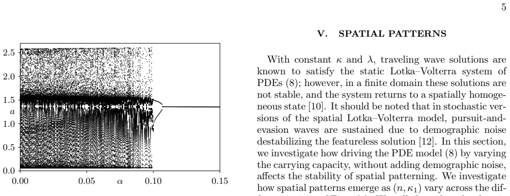
5 a FIG. 2: Value ofaat times that are an integer multiple of the period (the stroboscopic map), after a transient of 10000 periods for each parameter value in the ODEs (1). Parameter values area ∗ = 1,κ 0 = 0.25 and (n, κ1) = (0.7,0.24). Period-one orbits are represented by a single point, and period-two orbits, found below the period-doubling bifurcatio...
-
[5]
25 κ 1 FIG. 5: A parameter survey confirms the link between chaos in the mean-field ODEs (1) and the presence of spatial structure in the PDEs (8). The ODE data is the same as in, and the symbols have the same meaning as in, Fig. 1(c), though we have suppressed showing the period-one and period-two orbits. Red symbols indicate chaos in the ODEs, and the b...
-
[6]
A. J. Lotka,Elements of Physical Biology(Williams & Wilkins Co, Baltimore, 1925)
work page 1925
-
[7]
V. Volterra, Fluctuations in the abundance of a species considered mathematically, Nature118, 558 (1926)
work page 1926
-
[8]
J. D. Murray,Mathematical Biology: I. An Introduc- tion, Interdisciplinary Applied Mathematics, Vol. 17 (Springer, New York, NY, 2002)
work page 2002
-
[9]
Neal,Introduction to Population Biology, 2nd ed
D. Neal,Introduction to Population Biology, 2nd ed. (Cambridge University Press, Cambridge, 2018)
work page 2018
-
[10]
Maynard-Smith,Models in Ecology(Cambridge Uni- versity Press, Cambridge, 1978)
J. Maynard-Smith,Models in Ecology(Cambridge Uni- versity Press, Cambridge, 1978)
work page 1978
-
[11]
S. C. Bhargava, Generalized Lotka–Volterra equations and the mechanism of technological substitution, Tech- nological Forecasting and Social Change35, 319 (1989)
work page 1989
- [12]
-
[13]
C. Michalakelis, C. Christodoulos, D. Varoutas, and T. Sphicopoulos, Dynamic estimation of markets exhibit- ing a prey–predator behavior, Expert Systems with Ap- plications39, 7690 (2012)
work page 2012
-
[14]
V. W. Noonburg, A neural network modeled by an adap- tive Lotka–Volterra system, SIAM Journal on Applied Mathematics49, 1779 (1989)
work page 1989
-
[15]
S. R. Dunbar, Travelling wave solutions of diffusive Lotka–Volterra equations, Journal of Mathematical Bi- ology17, 11 (1983)
work page 1983
-
[16]
M. Mobilia, I. T. Georgiev, and U. C. T¨ auber, Phase transitions and spatio-temporal fluctuations in stochas- tic lattice Lotka–Volterra models, Journal of Statistical Physics128, 447 (2007)
work page 2007
-
[17]
U. Dobramysl, M. Mobilia, M. Pleimling, and U. C. T¨ auber, Stochastic population dynamics in spatially ex- tended predator–prey systems, Journal of Physics A: Mathematical and Theoretical51, 063001 (2018)
work page 2018
-
[18]
P. L. Chesson and R. R. Warner, Environmental variabil- ity promotes coexistence in lottery competitive systems, The American Naturalist117, 923 (1981)
work page 1981
-
[19]
R. M. May, Stability in randomly fluctuating versus de- 9 terministic environments, The American Naturalist107, 621 (1973)
work page 1973
-
[20]
T. Burkart, J. Willeke, and E. Frey, Periodic temporal environmental variations induce coexistence in resource competition models, Physical Review E108, 034404 (2023)
work page 2023
-
[21]
M. Rietkerk, S. C. Dekker, P. C. de Ruiter, and J. van de Koppel, Self-organized patchiness and catastrophic shifts in ecosystems, Science305, 1926 (2004)
work page 1926
-
[22]
T. Reichenbach, M. Mobilia, and E. Frey, Mobility pro- motes and jeopardizes biodiversity in rock-paper-scissors games, Nature448, 1046 (2007)
work page 2007
- [23]
- [24]
-
[25]
B. Bera, O. Tzuk, J. Bennett, U. Dieckmann, and E. Meron, Can spatial self-organization inhibit evolution- ary adaptation?, Journal of the Royal Society Interface 22, 20240454 (2025)
work page 2025
-
[26]
P. Gandhi, M. Oline, and M. Silber, A flow-kick model of dryland vegetation patterns: the impact of rainfall variability on resilience, arXiv preprint arXiv:2501.01569 10.48550/arXiv.2501.01569 (2025)
-
[27]
G. Floquet, Sur les ´ equations diff´ erentielles lin´ eaires ` a coefficients p´ eriodiques, Annales Scientifiques de l’´Ecole Normale Sup´ erieure12, 47 (1883)
-
[28]
S. H. Strogatz,Nonlinear Dynamics and Chaos, 2nd ed. (CRC Press, Boca Raton, 2015)
work page 2015
-
[29]
N. J. Balmforth, C. Pasquero, and A. Provenzale, The Lorenz–Fermi–Pasta–Ulam experiment, Physica D138, 1 (2000)
work page 2000
-
[30]
Y. Qian, H. Chen, and D.-H. Feng, Diffusive Lorenz dy- namics: Coherent structures and spatiotemporal chaos, Communications in Nonlinear Science and Numerical Simulation5, 49 (2000)
work page 2000
-
[31]
J. Hofbauer and K. Sigmund,Evolutionary Games and Population Dynamics(Cambridge University Press, Cambridge, 1998)
work page 1998
-
[32]
M. Swailem and U. C. T¨ auber, Lotka–Volterra predator- prey model with periodically varying carrying capacity, Physical Review E107, 064144 (2023)
work page 2023
-
[33]
L. Hern´ andez-Navarro, K. Distefano, U. C. T¨ auber, and M. Mobilia, Slow spatial migration can help eradicate cooperative antimicrobial resistance in time-varying en- vironments, BioRxiv preprint 10.1101/2024.12.30.630406 10.1101/2024.12.30.630406 (2024)
-
[34]
K. Wienand, E. Frey, and M. Mobilia, Evolution of a fluc- tuating population in a randomly switching environment, Physical Review Letters119, 158301 (2017)
work page 2017
-
[35]
K. Wienand, E. Frey, and M. Mobilia, Eco-evolutionary dynamics of a population with randomly switching carry- ing capacity, Journal of The Royal Society Interface15, 20180343 (2018)
work page 2018
-
[36]
A. Taitelbaum, R. West, M. Assaf, and M. Mobilia, Pop- ulation dynamics in a changing environment: Random versus periodic switching, Physical Review Letters125, 048105 (2020)
work page 2020
-
[37]
A. Taitelbaum, R. West, M. Mobilia, and M. Assaf, Evo- lutionary dynamics in a varying environment: Continu- ous versus discrete noise, Physical Review Research5, L022004 (2023)
work page 2023
- [38]
-
[39]
C. M. Bender and S. A. Orszag,Advanced Mathemati- cal Methods for Scientists and Engineers(McGraw–Hill, New York, 1978)
work page 1978
-
[40]
S. M. Cox and P. C. Matthews, Exponential time dif- ferencing for stiff systems, Journal of Computational Physics176, 430 (2002)
work page 2002
-
[41]
B. J. Walker, A. K. Townsend, A. K. Chudasama, and A. L. Krause, VisualPDE: Rapid interactive simulations of partial differential equations, Bulletin of Mathematical Biology85, 113 (2023)
work page 2023
-
[42]
Paramet- ric resonance, chaos and spatial structure in the Lotka– Volterra model
M. Swailem and A. M. Rucklidge, Dataset for “Paramet- ric resonance, chaos and spatial structure in the Lotka– Volterra model”, University of Leeds Data Repository (2025)
work page 2025
-
[43]
I. Kovacic, R. Rand, and S. M. Sah, Mathieu’s equation and its generalizations: Overview of stability charts and their features, Applied Mechanics Reviews70, 020802 (2018)
work page 2018
discussion (0)
Sign in with ORCID, Apple, or X to comment. Anyone can read and Pith papers without signing in.