REVIEW 5 major objections 5 minor 78 references
Figuring Out Gas & Galaxies In Enzo (FOGGIE). XIV. The Observability of Emission from Accretion and Feedback in the Circumgalactic Medium with Current and Future Instruments
T0 review · 5 major / 5 minor · reviewed 2026-08-03 · deepseek-v4-flash
Pith's one-line read For gas around galaxies, faintness—not blur—is the main detectability barrier; separating infall from outflow needs better than 30 km/s resolution.
desk verdict Solid sensitivity-vs-resolution trade study, but the 30 km/s inflow/outflow benchmark is likely overoptimistic because the kinematic metric ignores line widths. read the letter →
The pith
A machine-rendered reading of the paper's core claim, the machinery that carries it, and where it could break.
The reading
What carries the argument
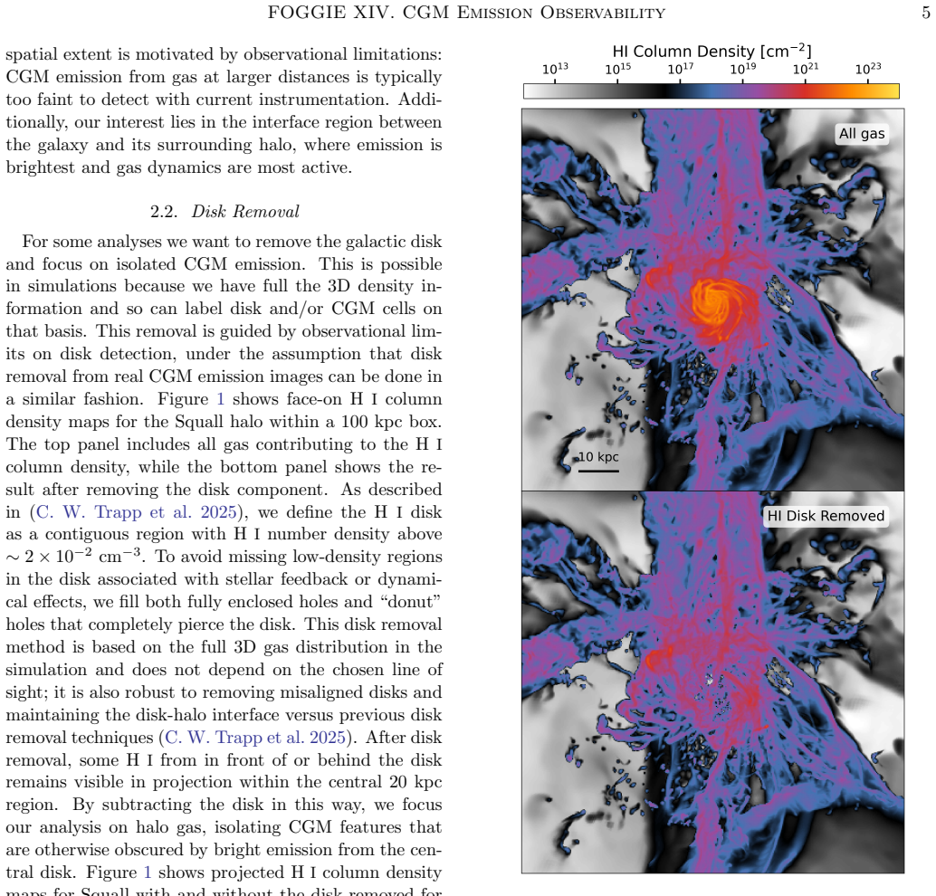
The central machinery is a mock-observation pipeline: eight emission lines (Hα, MgII, SiII, SiIII, CIII, CIV, SiIV, OVI) are assigned emissivities from photoionization-equilibrium tables as a function of local density, temperature, and metallicity; these are projected to surface-brightness and emissivity-weighted line-of-sight velocity maps for six simulated halos. A power-law fitting formula f=a x^b y^c then isolates the influence of spatial resolution x versus surface-brightness sensitivity y on recovered mass. A disk-removal step isolates the CGM from the galaxy's H I disk. Kinematic separability is quantified by thresholding pixel-by-pixel velocity differences at 300, 200, 100, and 30 km
What would settle it
A UV spectrograph reaching ≈100 photons s^-1 cm^-2 sr^-1 with ≈30 km/s resolution around a z≈0.5 galaxy could test the predictions: if the kinematically separable O VI area is much below 80% at 30 km/s, the kinematic claim fails. A rerun of the mass-fraction fits after including resonant-scattering radiative transfer for O VI and C IV would test whether c>b survives; if the sensitivity exponent drops below the resolution exponent, the central ranking is falsified.
Extended reading notes
Core claim
Surface-brightness sensitivity, not spatial resolution, controls how much circumgalactic (CGM) emitting mass an instrument recovers. Fitting recovered mass f=a x^b y^c to resolution x and sensitivity y gives c>b for all eight ions (≤7% error). Kinematically, emissivity-weighted projected velocity maps show that separating phases—and especially inflow (v≤-100 km/s) from outflow (v≥200 km/s)—requires ≲30 km/s: the separable bright area rises above 80% at 30 km/s and falls below 40% at 200 km/s. O VI traces diffuse warm-hot gas while Hα, MgII, and SiII trace cool clumps, so multi-ion mapping is essential.
Load-bearing premise
Every predicted map assumes the CGM is optically thin and in ionization equilibrium, with line emissivity taken from photoionization tables; because resonant scattering and radiative transfer are not modeled for lines like O VI, C IV, Mg II, and Si II, the predicted surface brightnesses—and therefore the sensitivity and 30 km/s benchmarks—could shift if scattered photons are suppressed or redistributed.
Editorial extensions
If this is right
- Future CGM emission mappers should be designed for surface-brightness limits near or below 500 photons s^-1 cm^-2 sr^-1; above that threshold the recoverable mass of diffuse high-ionization gas (O VI, C IV) drops sharply, so sensitivity is the first priority.
- Spectrographs should aim for delivered kinematic resolution around 30 km/s or finer: at 200 km/s less than 40% of the area of inflow/outflow overlap is separable, so coarse-resolution instruments cannot measure the inflow/outflow geometry of the CGM.
- No single emission line suffices: O VI, C IV, C III, Mg II, Si II, and Hα each highlight different phases and morphologies, so multi-ion wavelength coverage is needed to recover the multiphase CGM mass and kinematics.
- The observable mass fractions quoted are lower limits because the simulations underproduce ion column densities by 1–2 dex relative to quasar absorption observations; the ranking of sensitivity over resolution is unaffected by that normalization.
- Current facilities fall in different parts of the trade space—some reach the sensitivity regime, some reach the kinematic regime—so complementary observations with multiple instruments can cover the needed parameter space even if no single instrument does.
Reading between the lines
- Editorial inference: if resonant scattering (not modeled here) suppresses or redistributes light in the strong resonance lines O VI, C IV, Mg II, and Si II, the faint-end surface brightnesses—and hence the derived sensitivity and 30 km/s benchmarks—could move; a radiative-transfer post-processing test would quantify the shift.
- Editorial inference: the 30 km/s benchmark depends on the chosen inflow/outflow velocity cuts (≤-100 and ≥200 km/s); recomputing the separability fractions with different cuts, or with inflow/outflow defined by temperature or phase, would test how robust the >80%-at-30 km/s result is.
- Editorial inference: the method transfers to other masses and redshifts; dwarf galaxies and galaxy groups have lower-density, hotter CGM, where the sensitivity-dominance result could be even stronger and the required spectral resolution different.
Editorial analysis
A structured set of objections, weighed in public.
Referee Report
Summary. The paper uses six FOGGIE Milky Way-mass halos at z=0.5 to produce mock emission-line maps for eight UV/optical lines (Hα, MgII, SiII, CIII, SiIII, CIV, SiIV, OVI). It quantifies the observable CGM mass fraction as a function of spatial resolution and surface-brightness sensitivity, fits a power-law model f = a x^b y^c, and concludes that sensitivity is the dominant factor limiting detectability. It then constructs emissivity-weighted line-of-sight velocity maps and measures how well different ions, and inflowing versus outflowing gas, can be separated as a function of kinematic resolution, concluding that <30 km/s is required to distinguish inflow from outflow across more than 80% of the CGM area in all ions. Finally, it places current and proposed instruments in this parameter space and derives recommended sensitivity, spatial-resolution, and kinematic-resolution benchmarks.
Significance. If correct, the paper provides concrete, falsifiable instrument requirements for next-generation CGM emission mapping, and its multi-ion comparison is a useful step beyond single-line predictions. Strengths include the high-resolution FOGGIE sample, the explicit caveat that FOGGIE underpredicts column densities by 1–2 dex and that absolute mass fractions are lower limits, and the transparent emissivity pipeline with CLOUDY/CIAOLoop parameters in the appendix. The qualitative conclusion that sensitivity matters more than spatial resolution is directly visible in the heatmaps and is likely robust. However, the headline 30 km/s kinematic benchmark is not supported by the current analysis because the separation metric ignores line widths and spectral blending, and there are internal inconsistencies (HI versus Hα, UVB redshift) that must be addressed before the quantitative claims can be accepted.
major comments (5)
- [Section 5.2, Fig. 12] The 'distinguishable' criterion is only a comparison of emissivity-weighted mean velocities: |<v_in> - <v_out>| > R. It does not include intrinsic line widths, thermal/turbulent broadening, or spectral blending, even though the paper defines kinematic resolution as a 'delivered velocity separation between two components that can be reliably distinguished' in §5.1. A real observation yields a single blended spectrum; a 30 km/s centroid offset is not separable at 30 km/s resolution if the components have velocity dispersions of tens to hundreds of km/s. The headline claim that <30 km/s is required to distinguish inflow from outflow over more than 80% of the CGM area is therefore likely overoptimistic. Please recompute the fractions using synthetic spectra with realistic line profiles, or restate the result as a centroid-offset threshold rather than a distinguishability criterion.
- [Section 5.1, Figs. 8–9, abstract] The reference ion for the phase-kinematics comparison is called 'HI' throughout, but the line list (Table 2) and methods do not include an HI emission line; Hα is explicitly chosen instead of Lyα. If 'HI' is intended as neutral-hydrogen maps, the method for computing emissivity-weighted HI velocities is missing. If it is a typo for Hα, the interpretation that MgII and SiII 'follow HI velocities' is not supported, because Hα traces warm ionized gas rather than neutral gas. Please correct the notation and, if HI is intended, describe the calculation used to produce those maps.
- [Section 2.3 and Appendix C.0.1] The emissivity tables are constructed with the HM12 UV background at z=0 ('Table HM12 redshift 0.00', 'CMB redshift 0.00'), while the halos are analyzed at z=0.5. The text states that this is 'the same evolving UVB used during the simulation runtime,' which is contradictory: the simulation uses an evolving UVB, and at z=0.5 the ionizing background differs from z=0. This can bias ion-specific emissivities (e.g., MgII, SiII, CIV, OVI) and hence the mass-fraction fits and kinematic maps. Please recompute the tables at z=0.5 or justify quantitatively why the z=0 tables are adequate.
- [Section 2.3 and Section 5] All predictions assume optically thin line emission and neglect resonant scattering for the resonance lines considered (OVI 1032/1038, CIV 1548, MgII 2796, SiII 1260). At the low surface brightnesses of interest, resonant scattering can redistribute line photons and broaden line profiles, altering both the recovered mass fractions and the kinematic separability benchmarks. The paper justifies avoiding Lyα for this reason but does not assess the optical depth of the other lines. Please provide estimates of line-center optical depths in the simulated CGM, or a quantitative justification that these lines are effectively thin.
- [Section 4, Eq. (1), Fig. 6] The exponents b and c are reported without uncertainties or halo-to-halo scatter, and the fitting grid is coarse (4 spatial resolutions and a small number of sensitivity thresholds). The MAE ≤ 7% only measures how well the power law reproduces the grid values. To support the quantitative claim that 'sensitivity is dominant' and the corresponding abstract wording, please provide bootstrap or MCMC uncertainties and per-halo values, or restrict the claim to the qualitative trend that is directly visible in the heatmaps.
minor comments (5)
- [Section 2.3] The text says 'eight spectral lines: Hα, MgII, SiII, SiIII, CIII, CIV, and OVI,' which lists only seven lines; SiIV is missing. Please correct the list or the count.
- [Section 4, Fig. 5] The exact sensitivity grid values (100, 500, 2000, and any additional thresholds) are not stated in the text. Please specify the grid explicitly so the power-law fit is reproducible.
- [Section 5.2] The inflow/outflow definitions use asymmetric radial velocity cuts (-100 and +200 km/s). The results may depend on these cuts; please add a short robustness test or state clearly that the conclusions are conditional on this choice.
- [Section 7 and Fig. 12] The summary bullet says 'over 90%' of emission-resolved gas is kinematically distinguishable at 30 km/s, while Fig. 12 and the abstract state 'more than 80%.' Please harmonize these numbers and specify which quantity each refers to.
- [Table 3, Fig. 14] For MUSE and KCWI, the reported O VI and Hα surface-brightness limits are identical. Please clarify whether this is a deliberate simplification or a coincidence of the sensitivity calculation, since the sky background and throughput differ between the relevant redshift regimes.
Circularity Check
No significant circularity: results are forward-modeled from simulation post-processing; self-citations are methodological, not load-bearing.
full rationale
I walked the derivation chain. The central claims—sensitivity-limited detectability and the ~30 km/s kinematic-resolution requirement—are computed from FOGGIE simulation outputs via a fixed post-processing pipeline (CLOUDY emissivity tables, Trident ion masses, yt projections). Section 4's Eq. (1) is a descriptive power-law fit to the computed mass-fraction heatmaps; the conclusion that the sensitivity exponent c exceeds the resolution exponent b is a summary of those fitted values, not a target quantity defined by the fit. Section 5's 'distinguishable' criterion (|Δv| > resolution threshold) is an explicit, transparent definition; the resulting fractions are quantiles of the simulated centroid-difference maps, not a fitted parameter renamed as a prediction. The paper's self-citations (Corlies et al. 2020; Lochhaas et al. 2025; Trapp et al. 2025) establish the emissivity pipeline and disk-removal method; these are inherited methodology and are not invoked to forbid alternatives or to assert uniqueness. The paper also flags its own limitation (FOGGIE under-predicts column densities by 1–2 dex) and presents results as lower limits, further indicating the analysis is not constructed to force the conclusions. The skeptic's concern about ignoring line widths in the two-component separation is a correctness/physics limitation, not circularity: nothing in the paper's equations defines the target benchmark in terms of the model's free parameters.
Assumptions & free parameters
free parameters (5)
- Power-law exponents b and c =
per-ion b,c values from Eq. 1 (c>b for all ions)
- Power-law normalization a =
per-ion a from Eq. 1
- Inflow/outflow radial velocity cuts =
-100 km/s inflow, +200 km/s outflow
- HI disk removal density threshold =
n_HI ≈ 2e-2 cm^-3
- Surface brightness thresholds =
100, 500, 2000 photons s^-1 cm^-2 sr^-1
assumptions (7)
- domain assumption CGM line emission is dominated by collisional excitation followed by radiative decay, so emissivity scales as n_H^2 and can be precomputed from CLOUDY tables at given n_H, T, and redshift.
- domain assumption Each simulation cell is in ionization equilibrium under the Haardt & Madau (2012) UV background; photoionization and collisional ionization are included, non-equilibrium effects and local ionizing sources are not.
- domain assumption All metal-line emissivities scale linearly with cell metallicity from solar-metallicity CLOUDY tables.
- domain assumption The FOGGIE simulations with forced and cooling refinement reproduce the CGM density/temperature/metallicity structure well enough for observability trends; underpredictions of 1–2 dex in column density are acknowledged.
- domain assumption Six z=0.5 Milky Way-mass halos with no major mergers are representative of low-redshift CGM emission morphologies.
- domain assumption Projected emissivity-weighted velocity maps, binned to resolution thresholds, approximate what an integral-field spectrograph would measure; PSF and line-profile effects are ignored.
- ad hoc to paper Resonant scattering and radiative transfer are negligible for the UV/optical lines considered.
Cite this review
Pith. "Pith review of Figuring Out Gas & Galaxies In Enzo (FOGGIE). XIV. The Observability of Emission from Accretion and Feedback in the Circumgalactic Medium with Current and Future Instruments." pith.science (2026). https://pith.science/paper/34AXJCXG
@misc{pith2026251105644,
  author       = {Pith},
  title        = {Pith review of: Figuring Out Gas & Galaxies In Enzo (FOGGIE). XIV. The Observability of Emission from Accretion and Feedback in the Circumgalactic Medium with Current and Future Instruments},
  year         = {2026},
  howpublished = {\url{https://pith.science/paper/34AXJCXG}},
  note         = {Machine review of arXiv:2511.05644}
}
abstract
Observing the circumgalactic medium (CGM) in emission lines from ionized gas enables direct mapping of its spatial and kinematic structure, offering new insight into the gas flows that regulate galaxy evolution. Using the high-resolution Figuring Out Gas & Galaxies In Enzo (FOGGIE) simulations, we generate mock emission-line maps for six Milky Way-mass halos. Different lines (e.g., H$\alpha$, OVI) trace distinct CGM phases and structures, highlighting the importance of observations in multiple species. We quantify the observable CGM mass fraction as a function of instrument spatial resolution and surface brightness sensitivity, finding that sensitivity is the dominant factor limiting detectability across all ions. At fixed sensitivity, higher spatial resolution reveals more structures; at fixed spatial resolution, higher sensitivity recovers a higher percentage of the total mass. We explore CGM kinematics by constructing emissivity-weighted projected velocity maps and comparing line-of-sight velocities between emission lines. OVI shows the largest kinematic deviation from H$\alpha$, while MgII and SiII most closely follow HI velocities. Distinguishing these phases out to 50kpc from the galaxy center requires spectral resolution better than 30km/s for most ion pairs. Additionally, separating inflowing from outflowing gas based on projected kinematics also requires high spectral resolution: at 30km/s, more than 80% of gas above the emission detection threshold can be distinguished kinematically, but this fraction drops to <40% with a resolution of 200km/s. Our results provide predictions for future UV and optical instruments, showing that recovering the multiphase structure and kinematics of circumgalactic emission will require both high sensitivity and fine kinematic resolution.
Figures


Figures from the paper (14 more)


Reference graph
Works this paper leans on
-
[1]
Abraham, R. G., & van Dokkum, P. G. 2014, PASP, 126, 55, doi: 10.1086/674875
doi:10.1086/674875 2014
-
[2]
Acharyya, A., Peeples, M. S., Tumlinson, J., et al. 2024, arXiv e-prints, arXiv:2404.06613, doi: 10.48550/arXiv.2404.06613 Astropy Collaboration, Price-Whelan, A. M., Lim, P. L., et al. 2022, ApJ, 935, 167, doi: 10.3847/1538-4357/ac7c74
-
[3]
2021, MNRAS, 505, 6195, doi: 10.1093/mnras/stab1673
Augustin, R., P´ eroux, C., Hamanowicz, A., et al. 2021, MNRAS, 505, 6195, doi: 10.1093/mnras/stab1673
-
[4]
2019, MNRAS, 489, 2417, doi: 10.1093/mnras/stz2238
Augustin, R., Quiret, S., Milliard, B., et al. 2019, MNRAS, 489, 2417, doi: 10.1093/mnras/stz2238
-
[5]
Augustin, R., Tumlinson, J., Peeples, M. S., et al. 2025, arXiv e-prints, arXiv:2501.06551, doi: 10.48550/arXiv.2501.06551
-
[6]
Bahcall, J. N., & Spitzer, Jr., L. 1969, ApJL, 156, L63, doi: 10.1086/180350
doi:10.1086/180350 1969
-
[7]
Behroozi, P. S., Wechsler, R. H., & Wu, H.-Y. 2013, ApJ, 762, 109, doi: 10.1088/0004-637X/762/2/109
- [8]
Show all 78 references
-
[9]
J., Kacprzak, G
Bordoloi, R., Lilly, S. J., Kacprzak, G. G., & Churchill, C. W. 2014, ApJ, 784, 108, doi: 10.1088/0004-637X/784/2/108
2014 doi
-
[10]
M., Sharon, K., et al
Bordoloi, R., O’Meara, J. M., Sharon, K., et al. 2022, Nature, 606, 59, doi: 10.1038/s41586-022-04616-1
2022 doi
-
[11]
2016, ApJ, 833, 259, doi: 10.3847/1538-4357/833/2/259
Borthakur, S., Heckman, T., Tumlinson, J., et al. 2016, ApJ, 833, 259, doi: 10.3847/1538-4357/833/2/259
2016 doi
-
[12]
V., Chelouche, D., Jenkins, E
Bowen, D. V., Chelouche, D., Jenkins, E. B., et al. 2016, ApJ, 826, 50, doi: 10.3847/0004-637X/826/1/50
2016 doi
-
[13]
2019, The Journal of Open Source Software, 4, 1636, doi: 10.21105/joss.01636
Brummel-Smith, C., Bryan, G., Butsky, I., et al. 2019, The Journal of Open Source Software, 4, 1636, doi: 10.21105/joss.01636
2019 doi
-
[14]
L., Norman, M
Bryan, G. L., Norman, M. L., O’Shea, B. W., et al. 2014, ApJS, 211, 19, doi: 10.1088/0067-0049/211/2/19
2014 doi
-
[15]
P., et al
Cadiou, C., Katz, H., Rey, M. P., et al. 2025, arXiv e-prints, arXiv:2510.05667. https://arxiv.org/abs/2510.05667
2025
-
[16]
Cen, R., & Ostriker, J. P. 2006, ApJ, 650, 560, doi: 10.1086/506505
2006 doi
-
[17]
2023, RMxAA, 59, 327, doi: 10.22201/ia.01851101p.2023.59.02.12
Chatzikos, M., Bianchi, S., Camilloni, F., et al. 2023, RMxAA, 59, 327, doi: 10.22201/ia.01851101p.2023.59.02.12
2023 doi
-
[18]
M., Pasha, I., et al
Chen, S., Lokhorst, D. M., Pasha, I., et al. 2024, in Society of Photo-Optical Instrumentation Engineers (SPIE) Conference Series, Vol. 13094, Ground-based and Airborne Telescopes X, ed. H. K. Marshall, J. Spyromilio, & T. Usuda, 130942J, doi: 10.1117/12.3019491
2024 doi
-
[19]
M., Pasha, I., et al
Chen, S., Lokhorst, D. M., Pasha, I., et al. 2025, PASP, 137, 084103, doi: 10.1088/1538-3873/adedb8
2025 doi
-
[20]
J., & Hamden, E
Chung, H., Vargas, C. J., & Hamden, E. 2021a, ApJ, 916, 7, doi: 10.3847/1538-4357/ac04af
-
[22]
J., Hamden, E., et al
Chung, H., Vargas, C. J., Hamden, E., et al. 2021c, in Society of Photo-Optical Instrumentation Engineers (SPIE) Conference Series, Vol. 11819, UV/Optical/IR Space Telescopes and Instruments: Innovative Technologies and Concepts X, ed. A. A. Barto, J. B. Breckinridge, & H. P. ...
-
[23]
S., Tumlinson, J., et al
Corlies, L., Peeples, M. S., Tumlinson, J., et al. 2020, ApJ, 896, 125, doi: 10.3847/1538-4357/ab9310
2020 doi
-
[24]
L., & Mac Low, M.-M
Emerick, A., Bryan, G. L., & Mac Low, M.-M. 2019, MNRAS, 482, 1304, doi: 10.1093/mnras/sty2689 Faucher-Gigu` ere, C.-A., & Oh, S. P. 2023, ARA&A, 61, 131, doi: 10.1146/annurev-astro-052920-125203
2019 doi
-
[25]
P., Heckman, T., Strickland, D., et al
Grimes, J. P., Heckman, T., Strickland, D., et al. 2007, ApJ, 668, 891, doi: 10.1086/521353
2007 doi
-
[26]
Ha, T., Rupke, D. S. N., Caraker, S., et al. 2025, ApJ, 986, 87, doi: 10.3847/1538-4357/add0b5
2025 doi
-
[27]
2012, ApJ, 746, 125, doi: 10.1088/0004-637X/746/2/125
Haardt, F., & Madau, P. 2012, ApJ, 746, 125, doi: 10.1088/0004-637X/746/2/125
2012 doi
-
[28]
2016, ApJ, 828, 49, doi: 10.3847/0004-637X/828/1/49
Hayes, M., Melinder, J., ¨Ostlin, G., et al. 2016, ApJ, 828, 49, doi: 10.3847/0004-637X/828/1/49
2016 doi
-
[29]
B., Smith, B
Hummels, C. B., Smith, B. D., & Silvia, D. W. 2017, ApJ, 847, 59, doi: 10.3847/1538-4357/aa7e2d
2017 doi
-
[30]
B., Smith, B
Hummels, C. B., Smith, B. D., Hopkins, P. F., et al. 2019, ApJ, 882, 156, doi: 10.3847/1538-4357/ab378f
2019 doi
-
[31]
Hunter, J. D. 2007, Computing in Science and Engineering, 9, 90, doi: 10.1109/MCSE.2007.55
2007 doi
-
[32]
G., Churchill, C
Kacprzak, G. G., Churchill, C. W., & Nielsen, N. M. 2012, ApJL, 760, L7, doi: 10.1088/2041-8205/760/1/L7
2012 doi
-
[33]
J., & Hamden, E
Kim, J.-A., Chung, H., Vargas, C. J., & Hamden, E. 2024, AJ, 168, 11, doi: 10.3847/1538-3881/ad4887
2024 doi
-
[34]
J., D’Onghia, E., et al
Krishnarao, D., Fox, A. J., D’Onghia, E., et al. 2022, Nature, 609, 915, doi: 10.1038/s41586-022-05090-5
2022 doi
- [35]
-
[36]
2018, ApJ, 866, 36, doi: 10.3847/1538-4357/aadc08
Lan, T.-W., & Mo, H. 2018, ApJ, 866, 36, doi: 10.3847/1538-4357/aadc08
2018 doi
-
[37]
C., Tripp, T
Lehner, N., Howk, J. C., Tripp, T. M., et al. 2013, ApJ, 770, 138, doi: 10.1088/0004-637X/770/2/138
2013 doi
-
[38]
C., Howk, J
Lehner, N., Berek, S. C., Howk, J. C., et al. 2020, ApJ, 900, 9, doi: 10.3847/1538-4357/aba49c
2020 doi
- [40]
-
[41]
W., et al
Lochhaas, C., Tumlinson, J., O’Shea, B. W., et al. 2021, ApJ, 922, 121, doi: 10.3847/1538-4357/ac2496
2021 doi
-
[42]
S., et al
Lochhaas, C., Tumlinson, J., Peeples, M. S., et al. 2023, ApJ, 948, 43, doi: 10.3847/1538-4357/acbb06
2023 doi
-
[43]
S., O’Shea, B
Lochhaas, C., Peeples, M. S., O’Shea, B. W., et al. 2025, arXiv e-prints, arXiv:2510.25844. https://arxiv.org/abs/2510.25844
2025
-
[45]
2019b, ApJ, 877, 4, doi: 10.3847/1538-4357/ab184e
Schaye, J. 2019b, ApJ, 877, 4, doi: 10.3847/1538-4357/ab184e
-
[46]
F., et al
Lopez, S., Tejos, N., Barrientos, L. F., et al. 2020, MNRAS, 491, 4442, doi: 10.1093/mnras/stz3183 30Saeedzadeh et al
2020 doi
-
[47]
C., O’Sullivan, D., Matuszewski, M., et al
Martin, D. C., O’Sullivan, D., Matuszewski, M., et al. 2019, Nature Astronomy, 3, 822, doi: 10.1038/s41550-019-0791-2
2019 doi
-
[48]
M., Bacon, R., Bauer, S., et al
McDermid, R. M., Bacon, R., Bauer, S., et al. 2008, in 2007 ESO Instrument Calibration Workshop, ed. A. Kaufer & F. Kerber, 325, doi: 10.1007/978-3-540-76963-7 44
2008 doi
-
[49]
2024, ApJ, 974, 161, doi: 10.3847/1538-4357/ad6cd1
Melso, N., Schiminovich, D., Sitaram, M., et al. 2024, ApJ, 974, 161, doi: 10.3847/1538-4357/ad6cd1
2024 doi
-
[50]
2022, ApJ, 941, 185, doi: 10.3847/1538-4357/ac9d9c
Melso, N., Schiminovich, D., Smiley, B., et al. 2022, ApJ, 941, 185, doi: 10.3847/1538-4357/ac9d9c
2022 doi
-
[51]
M., Picouet, V., Lin, Z., et al
Miles, D. M., Picouet, V., Lin, Z., et al. 2025, ApJS, 278, 58, doi: 10.3847/1538-4365/add15c
2025 doi
-
[52]
C., et al
Morrissey, P., Matuszewski, M., Martin, D. C., et al. 2018, ApJ, 864, 93, doi: 10.3847/1538-4357/aad597
2018 doi
-
[53]
M., Churchill, C
Nielsen, N. M., Churchill, C. W., & Kacprzak, G. G. 2013, ApJ, 776, 115, doi: 10.1088/0004-637X/776/2/115
2013 doi
-
[54]
M., Fisher, D
Nielsen, N. M., Fisher, D. B., Kacprzak, G. G., et al. 2024, Nature Astronomy, 8, 1602, doi: 10.1038/s41550-024-02365-x
2024 doi
-
[55]
M., Howk, J
Otte, B., Murphy, E. M., Howk, J. C., et al. 2003, ApJ, 591, 821, doi: 10.1086/375535
2003 doi
-
[56]
S., Werk, J
Peeples, M. S., Werk, J. K., Tumlinson, J., et al. 2014, ApJ, 786, 54, doi: 10.1088/0004-637X/786/1/54
2014 doi
-
[57]
S., Corlies, L., Tumlinson, J., et al
Peeples, M. S., Corlies, L., Tumlinson, J., et al. 2019, ApJ, 873, 129, doi: 10.3847/1538-4357/ab0654 Planck Collaboration, Ade, P. A. R., Aghanim, N., et al. 2016, A&A, 594, A13, doi: 10.1051/0004-6361/201525830
2019 doi
-
[58]
2018, ApJS, 237, 23, doi: 10.3847/1538-4365/aac832
Pontzen, A., & Tremmel, M. 2018, ApJS, 237, 23, doi: 10.3847/1538-4365/aac832
2018 doi
-
[59]
X., Werk, J
Prochaska, J. X., Werk, J. K., Worseck, G., et al. 2017, ApJ, 837, 169, doi: 10.3847/1538-4357/aa6007
2017 doi
-
[60]
M., et al
Shaban, A., Bordoloi, R., O’Meara, J. M., et al. 2025, ApJ, 986, 190, doi: 10.3847/1538-4357/add0b9
2025 doi
-
[61]
C., Peeples, M
Simons, R. C., Peeples, M. S., Tumlinson, J., et al. 2020, ApJ, 905, 167, doi: 10.3847/1538-4357/abc5b8
2020 doi
- [62]
-
[63]
Norman, M. L. 2009, ApJ, 691, 441, doi: 10.1088/0004-637X/691/1/441
2009 doi
-
[64]
D., Bryan, G
Smith, B. D., Bryan, G. L., Glover, S. C. O., et al. 2017, MNRAS, 466, 2217, doi: 10.1093/mnras/stw3291
2017 doi
- [65]
-
[66]
W., Peeples, M
Trapp, C. W., Peeples, M. S., Tumlinson, J., et al. 2025, arXiv e-prints, arXiv:2511.00158. https://arxiv.org/abs/2511.00158
2025 arXiv
-
[67]
S., & Werk, J
Tumlinson, J., Peeples, M. S., & Werk, J. K. 2017, ARA&A, 55, 389, doi: 10.1146/annurev-astro-091916-055240
2017 doi
-
[68]
K., et al
Tumlinson, J., Thom, C., Werk, J. K., et al. 2011, Science, 334, 948, doi: 10.1126/science.1209840
2011 doi
-
[69]
K., et al
Tumlinson, J., Thom, C., Werk, J. K., et al. 2013, ApJ, 777, 59, doi: 10.1088/0004-637X/777/1/59
2013 doi
-
[70]
J., Smith, B
Turk, M. J., Smith, B. D., Oishi, J. S., et al. 2011, The Astrophysical Journal Supplement Series, 192, 9, doi: 10.1088/0067-0049/192/1/9 van de Voort, F., Springel, V., Mandelker, N., van den
2011 doi
-
[71]
C., & Pakmor, R
Bosch, F. C., & Pakmor, R. 2019, MNRAS, 482, L85, doi: 10.1093/mnrasl/sly190
2019 doi
-
[72]
E., et al
Virtanen, P., Gommers, R., Oliphant, T. E., et al. 2020, Nature Methods, 17, 261, doi: 10.1038/s41592-019-0686-2
2020 doi
-
[73]
2025, in American Astronomical Society Meeting Abstracts, Vol
Vorobiev, D. 2025, in American Astronomical Society Meeting Abstracts, Vol. 246, 246th Meeting of the American Astronomical Society, 141.03
2025
-
[74]
Walt, S. v. d., Colbert, S. C., & Varoquaux, G. 2011, Computing in Science & Engineering, 13, 22
2011
-
[75]
2021, MNRAS, 502, 3733, doi: 10.1093/mnras/stab049
Muzahid, S. 2021, MNRAS, 502, 3733, doi: 10.1093/mnras/stab049
2021 doi
-
[76]
K., Prochaska, J
Werk, J. K., Prochaska, J. X., Tumlinson, J., et al. 2014, ApJ, 792, 8, doi: 10.1088/0004-637X/792/1/8
2014 doi
-
[77]
2018, Nature, 562, 229, doi: 10.1038/s41586-018-0564-6
Wisotzki, L., Bacon, R., Brinchmann, J., et al. 2018, Nature, 562, 229, doi: 10.1038/s41586-018-0564-6
2018 doi
-
[78]
M., Fleming, B
Witt, E. M., Fleming, B. T., McCandliss, S., et al. 2025, in
2025
-
[79]
C., Tumlinson, J., Peeples, M
Wright, A. C., Tumlinson, J., Peeples, M. S., et al. 2024, ApJ, 970, 70, doi: 10.3847/1538-4357/ad49a3
2024 doi
-
[80]
S., Chen, H.-W., Johnson, S
Zahedy, F. S., Chen, H.-W., Johnson, S. D., et al. 2019, MNRAS, 484, 2257, doi: 10.1093/mnras/sty3482
2019 doi
-
[81]
S., O’Shea, B
Zheng, Y., Peeples, M. S., O’Shea, B. W., et al. 2020, ApJ, 896, 143, doi: 10.3847/1538-4357/ab960a
2020 doi
Reviewed August 3, 2026 · model on record in the stance chip above.
Discussion (0). Sign in to comment.