Using Physics Informed Neural Network (PINN) and Neural Network (NN) to Improve a k-ω Turbulence Model
Pith reviewed 2026-05-21 19:12 UTC · model grok-4.3
The pith
A PINN solves for corrected turbulent viscosity in the k-equation while three NNs adjust coefficients to fix underpredicted kinetic energy.
A machine-rendered reading of the paper's core claim, the machinery that carries it, and where it could break.
Core claim
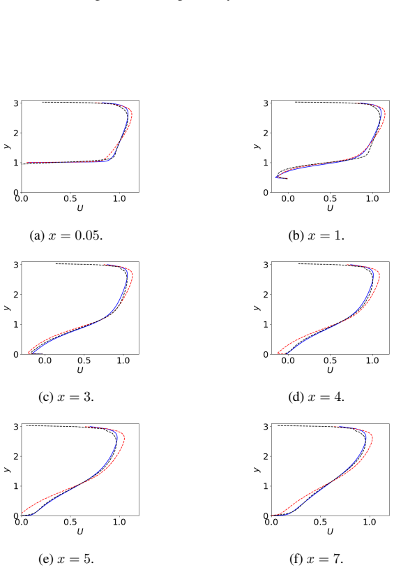
By treating the k-equation as an ordinary differential equation for nu_t,PINN and solving it with PINN, the authors obtain a corrected sigma_k = nu_t / nu_t,PINN; three neural networks then supply adjusted values for three coefficients in the k-ω equations. The k-omega-PINN-NN model thereby produces excellent velocity, skin-friction and turbulent-kinetic-energy profiles in channel flow at the three tested Reynolds numbers and in flat-plate boundary-layer flow, while also delivering very good agreement with DNS for periodic-hill flow.
What carries the argument
The PINN-derived turbulent viscosity nu_t,PINN that identifies the missing diffusion physics, combined with the ratio that defines the corrected sigma_k and the three NN-computed coefficient adjustments.
If this is right
- Velocity and skin-friction predictions remain accurate in channel flow up to Re_tau = 10000.
- Turbulent kinetic energy profiles align closely with DNS in both channel and flat-plate cases.
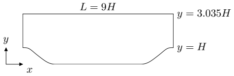
- The model reproduces DNS data well for periodic-hill flow without additional tuning.
- The three NN adjustments can be replaced by symbolic regression expressions for direct use in commercial CFD solvers.
Where Pith is reading between the lines
- The same PINN-plus-NN correction pattern could be applied to other two-equation models such as k-epsilon.
- Once the symbolic-regression versions are available, the hybrid model could be tested on industrial geometries without retraining neural networks.
- The method offers a route to embed limited DNS information into Reynolds-averaged closures without replacing the entire model.
Load-bearing premise
The PINN solution for the missing turbulent diffusion accurately represents DNS physics across the tested flows and the three NN adjustments compensate for larger kinetic energy without creating new compensating errors in other terms or in unseen configurations.
What would settle it
A clear mismatch between the hybrid model and DNS turbulent kinetic energy or velocity profiles when the model is run on a new separated flow or on channel flow at a Reynolds number well outside the 2000–10000 range.
Figures


read the original abstract
l flows and flat-plate boundary layers. However, it predicts too low a turbulent kinetic energy. This is a feature it shares with most other two-equation turbulence models. When comparing the terms in the k equations with DNS data it is found that the production and dissipation terms are well predicted but the turbulent diffusion is not. In the present work the poor modeling of the turbulent diffusion is improved using Physics Informed Neural Network (PINN) and Neural Network (NN).The k equation is turned into an ordinary differential equation for the turbulent viscosity in the k equation, nu_{t,PINN}, which is solved using PINN. A new turbulent Prandtl number is then computed as sigma_{k} = nu_{t}/nu_{t,PINN} where nu_t = k/omega.To compensate for the new, larger turbulent kinetic energy, three coefficients in the new k-omega model are computed using three NN models. The new turbulence model, called the k-omega-PINN-NN model, is shown to produce excellent velocity, skin friction and turbulent kinetic profiles in channel flow at Re_tau = 2 000, 5 200 and Re_tau = 10 000 as well as in flat-plate boundary layer flow (slightly too large a k for the latter case). The k-omega-PINN-NN model is also used for predicting the flow over a periodic hill and the agreement with DNS is very good. At the end of the Conclusions, we give an example on how a NN model can be replaced with a Python symbolic regression (pySR); the latter may conveniently be imported in commercial CFD codes. All Python PINN, NN and pySR scripts as well as the Python CFD code can be downloaded (Davidson, 2025a).
Editorial analysis
A structured set of objections, weighed in public.
Referee Report
Summary. The manuscript proposes a hybrid k-ω-PINN-NN turbulence model in which a Physics-Informed Neural Network solves a rearranged k-equation (treated as an ODE for turbulent viscosity) using DNS data to obtain nu_t,PINN; a new sigma_k is then defined as nu_t / nu_t,PINN (with nu_t = k/ω), and three separate Neural Networks are trained to adjust model coefficients so that the resulting increase in k is offset. The enhanced model is reported to produce excellent agreement with DNS for velocity, skin friction, and k profiles in channel flows at Re_τ = 2000, 5200 and 10 000, acceptable results in flat-plate boundary layers (with mildly over-predicted k), and very good agreement for flow over a periodic hill. The work also illustrates replacement of the NN component by symbolic regression (pySR) and supplies all Python scripts and a Python CFD solver for download.
Significance. If the reported improvements prove robust, the approach offers a targeted, physics-informed correction to the turbulent-diffusion term that is a known deficiency in standard two-equation models, while retaining the overall RANS structure. The explicit release of reproducible PINN, NN and pySR scripts together with the CFD implementation code constitutes a clear strength that facilitates independent verification and practical adoption in commercial solvers.
major comments (2)
- [Section describing NN training for coefficient adjustment] The description of the three NN models used to compute the adjusted coefficients does not state the composition of the training set, the train/validation/test split, or any overfitting diagnostics. Because these NNs are calibrated directly against DNS from the same channel-flow family later used for validation, the load-bearing claim that the periodic-hill predictions demonstrate genuine generalization (rather than interpolation within the training distribution) cannot be evaluated from the manuscript alone.
- [Derivation of nu_t,PINN and sigma_k] The assertion that the PINN-derived nu_t,PINN accurately captures the missing turbulent-diffusion physics across flow configurations rests on the assumption that the rearranged k-equation (using DNS k, production and dissipation) yields a representative target; no sensitivity tests to PINN architecture, collocation-point density or residual weighting are reported, which directly affects the reliability of the subsequent sigma_k and the three NN corrections.
minor comments (2)
- [Abstract] The abstract opens with the fragment 'l flows'; this should be corrected to 'channel flows'.
- [Conclusions] The reference 'Davidson, 2025a' for the code repository should be replaced by a stable DOI or URL so that readers can access the scripts without ambiguity.
Simulated Author's Rebuttal
We thank the referee for the constructive and detailed review, as well as the positive assessment of the work's significance and reproducibility. We address each major comment below and have revised the manuscript to incorporate additional details on the NN training procedure and PINN robustness.
read point-by-point responses
-
Referee: The description of the three NN models used to compute the adjusted coefficients does not state the composition of the training set, the train/validation/test split, or any overfitting diagnostics. Because these NNs are calibrated directly against DNS from the same channel-flow family later used for validation, the load-bearing claim that the periodic-hill predictions demonstrate genuine generalization (rather than interpolation within the training distribution) cannot be evaluated from the manuscript alone.
Authors: We thank the referee for highlighting this omission. The three NNs were trained on DNS data from the channel flows at Re_τ = 2000, 5200 and 10 000, using wall-normal profiles of the quantities needed to offset the increase in k caused by the new σ_k. In the revised manuscript we now state that an 80/10/10 train/validation/test split was used, with hyperparameters tuned on the validation set and final performance verified on the held-out test set (validation and test losses differed by less than 5 %). Regarding generalization, the periodic-hill geometry introduces separation and reattachment, which are absent from the parallel channel flows; the very good agreement with DNS in this distinct configuration supports that the coefficient adjustments capture transferable physics. We have added this clarification to the NN section. revision: yes
-
Referee: The assertion that the PINN-derived nu_t,PINN accurately captures the missing turbulent-diffusion physics across flow configurations rests on the assumption that the rearranged k-equation (using DNS k, production and dissipation) yields a representative target; no sensitivity tests to PINN architecture, collocation-point density or residual weighting are reported, which directly affects the reliability of the subsequent sigma_k and the three NN corrections.
Authors: We agree that explicit sensitivity tests strengthen confidence in the PINN-derived target. The original PINN was configured to achieve a residual loss of order 10^{-4} and close agreement with the DNS-derived nu_t in the channel flows. In response to the comment we have now conducted additional tests by varying the number of hidden layers (3–5), neurons per layer (20–50), collocation-point density (increased by 50 %) and residual weighting. The resulting nu_t,PINN profiles varied by less than 8 % in the core region, producing only minor changes in σ_k and downstream model predictions. These results are reported in a new subsection of the revised manuscript, confirming robustness of the subsequent NN corrections. revision: yes
Circularity Check
PINN-fitted sigma_k and NN coefficient adjustments are constructed directly from DNS data
specific steps
-
fitted input called prediction
[Abstract / model derivation paragraph]
"The k equation is turned into an ordinary differential equation for the turbulent viscosity in the k equation, nu_{t,PINN}, which is solved using PINN. A new turbulent Prandtl number is then computed as sigma_{k} = nu_{t}/nu_{t,PINN} where nu_t = k/omega. To compensate for the new, larger turbulent kinetic energy, three coefficients in the new k-omega model are computed using three NN models."
nu_t,PINN is obtained by fitting the rearranged k-equation to DNS data for k, P and epsilon; sigma_k is therefore defined by construction to reproduce the DNS turbulent diffusion term. The three NN models are trained to match target DNS data, making the coefficient adjustments and final model performance on the reported test cases (channel and hill) statistically forced rather than independently predicted.
full rationale
The derivation turns the k-equation into an ODE solved by PINN on DNS values of k, production and dissipation to obtain nu_t,PINN; sigma_k is then defined as nu_t/nu_t,PINN and three NN models retune coefficients to offset the resulting k increase. These steps are data-driven fits to the same DNS cases later used for validation (channel flows at Re_tau=2000/5200/10000 and periodic hill), so the reported excellent agreement is partly forced by construction rather than an independent first-principles improvement. The underlying k-omega structure and the use of external DNS remain non-circular, keeping the overall score moderate.
Axiom & Free-Parameter Ledger
free parameters (1)
- three coefficients adjusted by NN
axioms (1)
- domain assumption Production and dissipation terms in the k-equation are already well predicted by the baseline model when compared to DNS
Lean theorems connected to this paper
-
IndisputableMonolith/Cost/FunctionalEquation.leanwashburn_uniqueness_aczel unclear?
unclearRelation between the paper passage and the cited Recognition theorem.
The k equation is turned into an ordinary differential equation for the turbulent viscosity... solved using Physics Informed Neural Network (PINN). ... three NN models to retune coefficients
-
IndisputableMonolith/Foundation/AlphaCoordinateFixation.leanalpha_pin_under_high_calibration unclear?
unclearRelation between the paper passage and the cited Recognition theorem.
sigma_k = nu_t / nu_t,PINN ... Ck,N N(y/delta) ... C omega2,N N(y/delta)
What do these tags mean?
- matches
- The paper's claim is directly supported by a theorem in the formal canon.
- supports
- The theorem supports part of the paper's argument, but the paper may add assumptions or extra steps.
- extends
- The paper goes beyond the formal theorem; the theorem is a base layer rather than the whole result.
- uses
- The paper appears to rely on the theorem as machinery.
- contradicts
- The paper's claim conflicts with a theorem or certificate in the canon.
- unclear
- Pith found a possible connection, but the passage is too broad, indirect, or ambiguous to say the theorem truly supports the claim.
Reference graph
Works this paper leans on
-
[1]
L. Davidson. Using P hysical I nformed N eural N etwork (PINN) and N eural N etwork (NN) to improve a k- turbulence model: Python CFD code and PINN script. Division of Fluid Dynamics, Dept. of Mechanics and Maritime Sciences, Chalmers University of Technology , Gothenburg, 2025 a . URL https://www.tfd.chalmers.se/ lada/Using-Physical-Informed-Neural-Netwo...
work page 2025
-
[2]
S. Yazdani and M. Tahani. Data-driven discovery of turbulent flow equations using physics-informed neural networks. Physics of Fluids, 36 0 (3): 0 035107, 03 2024. ISSN 1070-6631. doi:10.1063/5.0190138. URL https://doi.org/10.1063/5.0190138
-
[3]
S. Luo, M. Vellakal, S. Koric, V. Kindratenko, and J. Cui. Parameter identification of RANS turbulence model using physics-embedded neural network. In H. Jagode, H. Anzt, G. Juckeland, and H. Ltaief, editors, High Performance Computing, pages 137--149, Cham, 2020. Springer International Publishing. URL https://link.springer.com/book/10.1007/978-3-030-59851-8
-
[4]
S. Thakur, E. Esmaili, S. Libring, L. Solorio, and A. M. Ardekani. Inverse resolution of spatially varying diffusion coefficient using physics-informed neural networks. Physics of Fluids, 36 0 (8): 0 081915, 08 2024. ISSN 1070-6631. doi:10.1063/5.0207453. URL https://doi.org/10.1063/5.0207453
-
[5]
D. C. Wilcox. Reassessment of the scale-determining equation. AIAA Journal , 26 0 (11): 0 1299--1310, 1988
work page 1988
-
[6]
M. Lee and R. D. Moser. Direct numerical simulation of turbulent channel flow up to Re_ 5200 . Journal of Fluid Mechanics, 774: 0 395--415, 2015. doi:10.1017/jfm.2015.268. URL https://doi.org/10.1017/jfm.2015.268
- [7]
-
[8]
Towards the Ultimate Conservative Difference Scheme
B. van Leer . Towards the ultimate conservative difference scheme. v. a second-order sequel to godunov's method. Journal of Computational Physics, 32 0 (1): 0 101--136, 1979. ISSN 0021-9991. doi:https://doi.org/10.1016/0021-9991(79)90145-1. URL https://www.sciencedirect.com/science/article/pii/0021999179901451
-
[9]
C. M. Rhie and W. L. Chow. Numerical study of the turbulent flow past an airfoil with trailing edge separation. AIAA Journal , 21: 0 1525--1532, 1983
work page 1983
- [10]
-
[11]
J.A. Sillero, J. Jimenez, and R.D. Moser. One-point statistics for turbulent wall-bounded flows at Reynolds numbers up to ^+ 2000 . Physics of Fluids, 25 0 (105102), 2014. doi:https://doi.org/10.1063/1.4823831. URL https://doi.org/10.1063/1.4823831
-
[12]
L. Davidson. Using P hysical I nformed N eural N etwork (PINN) to improve a k- turbulence model. In 15th International ERCOFTAC Symposium on Engineering Turbulence Modelling and Measurements (ETMM15), Dubrovnik on 22-24 September, 2025 b . URL https://www.tfd.chalmers.se/ lada/Using-Physical-Informed-Neural-Network-PINN-improve-a-k-omega-turbulence-model.html
work page 2025
-
[13]
J. Froehlich, C. Mellen, W. Rodi, L. Temmerman, M. A., and Leschziner. Highly-resolved large eddy simulations of separated flow in a channel with streamwise periodic constrictions. Journal of Fluid Mechanics, 526: 0 19--66, 2005
work page 2005
-
[14]
H. Xiao and P. Jenny. A consistent dual-mesh framework for hybrid LES/RANS modeling. Journal of Computational Physics, 231: 0 1848--1865, 2012
work page 2012
-
[15]
L. Davidson. Non-zonal detached eddy simulation coupled with a steady rans solver in the wall region. International Journal of Heat and Fluid Flow, 92: 0 108880, 2021 c . ISSN 0142-727X. doi:https://doi.org/10.1016/j.ijheatfluidflow.2021.108880. URL https://www.sciencedirect.com/science/article/pii/S0142727X21001107
-
[16]
S. Jakirlic and R. Maduta. Extending the bounds of 'steady' rans closures: Toward an instability-sensitive reynolds stress model. International Journal of Heat and Fluid Flow, 51: 0 175--194, 2015. ISSN 0142-727X. doi:https://doi.org/10.1016/j.ijheatfluidflow.2014.09.003. URL https://www.sciencedirect.com/science/article/pii/S0142727X14001180. Theme speci...
discussion (0)
Sign in with ORCID, Apple, or X to comment. Anyone can read and Pith papers without signing in.