pith. sign in

arxiv: 2511.15893 · v2 · pith:IHVWGEPKnew · submitted 2025-11-19 · 🧮 math.PR

On a Class of Dynamical Poisson-Voronoi Tessellations

Pith reviewed 2026-05-21 17:51 UTC · model grok-4.3

classification 🧮 math.PR
keywords dynamical Poisson-Voronoi tessellationhandover point processstationarityMarkovian dynamicsinter-event timesPalm distributionmobile stationssatellite communication model
0
0 comments X

The pith

Dynamical Poisson-Voronoi tessellations from moving stations yield a stationary handover point process whose intensity and inter-event times are explicitly determined.

A machine-rendered reading of the paper's core claim, the machinery that carries it, and where it could break.

The paper examines a model where mobile stations start at random positions given by a Poisson point process and move at constant speeds in random directions across the plane. Fixed users connect to the nearest station at each moment, causing handovers as stations move and the closest one changes. The authors prove that the sequence of these handover times for a typical user forms a stationary point process on the time line. They compute its intensity, the joint distribution of the times between handovers, and several Palm distributions at handover moments, including distances to nearby stations. This applies to both uniform speeds and mixtures of speeds, and identifies a three-dimensional Markov state that captures the future evolution of associations.

Core claim

In this dynamical Poisson-Voronoi model, the handover point process observed by a typical fixed user is stationary. Its intensity is derived explicitly, as is the joint distribution of successive inter-handover intervals. The process admits a three-dimensional state description consisting of the distance to the serving station, the distance to the next nearest, and the relative velocities, which renders the association dynamics Markovian. These properties hold in both the single-speed and multi-speed cases.

What carries the argument

The handover point process, defined as the epochs when a typical user switches to a new nearest mobile station, together with the three-dimensional state variables that Markovize the association dynamics.

Load-bearing premise

The stations begin at positions drawn from a homogeneous Poisson point process and each moves forever at its own fixed speed in a uniformly random direction.

What would settle it

Simulate many trajectories of Poisson-initialized stations moving at constant speeds; count the number of handovers per unit time for a fixed user and check whether it converges to the paper's predicted intensity value.

Figures

Figures reproduced from arXiv: 2511.15893 by Fran\c{c}ois Baccelli, Sanjoy Kumar Jhawar.

Figure 3
Figure 3. Figure 3: as guiding line, while also indicating the key geometric objects of interest in the single-speed [PITH_FULL_IMAGE:figures/full_fig_p005_3.png] view at source ↗
Figure 3.1
Figure 3.1. Figure 3.1: Summary for the handover process in the single-speed case. We also study the point process of visible heads (this correspond to the ‘best’ location of the serving station), depicted by in [PITH_FULL_IMAGE:figures/full_fig_p006_3_1.png] view at source ↗
Figure 3.2
Figure 3.2. Figure 3.2: Summary for the handover process in the two-speed case. 3.3. Sequential organization of the article. The organization of the rest of the article is as fol￾lows. In Section 4, we first set up the ground work for defining the radial bird particle process and it’s fundamental properties that will be used in deriving our result about handover frequency in Theo￾rem 4.26. The heart of the problem lies in deter… view at source ↗
Figure 4.1
Figure 4.1. Figure 4.1: Properties of the distance function. 3. Family of curves: Fix some s ∈ R. For u ∈ R +, gs,u(t) := |(t, 0) − (s, u)| is the height at time t of the bird with head at (s, u). Then {gs,u(·)}u∈R+ defines the set of all radial birds with head at (s, u) when varying u ∈ R +. Each element in this family has the lines h = s + t and h = s − t, for h ∈ R +, as its asymptotes (see Picture 2 of [PITH_FULL_IMAGE:fig… view at source ↗
Figure 4.2
Figure 4.2. Figure 4.2: The birds together with their heads form the radial bird particle process Pc ≡ Hc. Proof of Lemma 4.11 (i). There is a bijection between the atom (Ri , αi), the corresponding radial bird Ci ≡ C(Ri,αi) and its head (Ti , Hi). The proof then follows from the inverse construction of set valued marked Poisson point process from the set process described in [3, Proposition 10.2.10], using the Poisson point pr… view at source ↗
Figure 4.3
Figure 4.3. Figure 4.3: The blue ×’s forms the handover point process on the time-axis. The blue nodes (•), block nodes (•) and red nodes (•), respectively, on individual vertical blue, black and red lines, respectively, forms the point process corresponding to the distance of all the mobile base stations at handover times, at a time corresponding to a head and at a typical time, respectively. Having defined the radial bird par… view at source ↗
Figure 4.4
Figure 4.4. Figure 4.4: Scenario in Observation 4.17. All birds with head point inside and outside, respectively, of the half-ball of height h ′ , intersect the vertical line below and above the level h ′ , respectively. Lemma 4.18. For any point (t, h) ∈ ∪i∈NCi, the following holds: (i). The point (t, h) belongs to Le if and only if H(U t h ) = 0, where H is the head point process. (ii). The probability of such an event is P((… view at source ↗
Figure 4.5
Figure 4.5. Figure 4.5: The two scenarios of (0, h) being or not being a head point. Case 2: (0, h) is not a head point. Suppose (0, h) is any other point of C ′ than its head, as in Figure (4.5) (Picture 2). Let (s, u) be a point on ∂ ∗Uh. Using the same argument as in case (5), one can prove that the radial bird with its head at (s, u) passes through (0, h). Due to Observation 4.17, any other radial bird with its heads inside… view at source ↗
Figure 4
Figure 4. Figure 4: (Picture 1)). This implies that any other radial bird with its head inside [PITH_FULL_IMAGE:figures/full_fig_p014_4.png] view at source ↗
Figure 4.6
Figure 4.6. Figure 4.6: (Picture 1)). This implies that any other radial bird with its head inside Uh intersects the height-axis below the level h, and this prevents (0, h) from being a handover point. As a consequence, we have that H(Uh) = 0. t (0, h) • • (1) The semicircle of radius h, passing through the in￾tersection of two birds, passes through their heads, for any pair of birds. For (0, h) to be a handover point, the regi… view at source ↗
Figure 4
Figure 4. Figure 4: (Picture 2). For any [PITH_FULL_IMAGE:figures/full_fig_p015_4.png] view at source ↗
Figure 4.7
Figure 4.7. Figure 4.7: Construction of the handover point process V and its marked version Vˆ. Let (t, h) ̸= (t ′ , h′ ) ∈ H+ be such that t ′ < t and the corresponding radial birds C(t,h) , C(t ′ ,h′) intersect at (ˆs, hˆ). The quantities ˆs and hˆ are derived later in (4.22) and (4.23), respectively, in terms of (t, h),(t ′ , h′ ). Let A(ˆs, hˆ) be the event that the intersection point (ˆs, hˆ) represents a handover. By Lemm… view at source ↗
Figure 4.8
Figure 4.8. Figure 4.8: Given (t, h) and (t ′ , h′ ), the intersection (ˆs, hˆ) is a handover point if and only if H(U sˆ hˆ ) = 0. We have the following result about the independence of the head point processes restricted to U sˆ hˆ and (U sˆ hˆ ) c , under the two point Palm probability measure P (t,h,C),(t ′ ,h′ ,C′ ) Hc . We state it as a corollary without proof, as it directly follows from the fact that Poisson point proce… view at source ↗
Figure 4.9
Figure 4.9. Figure 4.9: In the dual system the handover points are represented by the crossings of the Voronoi boundaries by the trajectory of an user moving along a horizontal line. 19 [PITH_FULL_IMAGE:figures/full_fig_p019_4_9.png] view at source ↗
Figure 4.10
Figure 4.10. Figure 4.10: All the radial birds intersects the line Ls at different heights and creates a point process ηs. Then hˆ s is the distance to the serving station at time s, which characterizes the power of the signal received by the user. On the other hand the point process ηs − δ hˆs enables us to encode the distance of all other non-serving stations, contributing to the power of the interference experienced by the us… view at source ↗
Figure 5.1
Figure 5.1. Figure 5.1: The bijection between point process R and the handover point process V via the head point process H and the intersection points of the radial birds. V, that will be denoted by β, (see [PITH_FULL_IMAGE:figures/full_fig_p022_5_1.png] view at source ↗
Figure 5.2
Figure 5.2. Figure 5.2: The mobile station, corresponding to the radial bird in red, partly serves the user, but not during the time when it is at its closest distance. Remark 5.10. The point process HV consists of only those atoms of H that lie on the lower envelope. There can be some atoms of H for which a part of the corresponding radial bird contributes to the lower envelope, but are such that the head point itself does not… view at source ↗
Figure 5.3
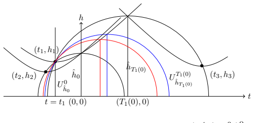
Figure 5.3. Figure 5.3: The sequence of increasing sets of the form St = (U t hˆt \ U 0 hˆ0 ) o has no points of H, for all t ∈ [0, T1(0)], we just draw a two of them in red and blue. Here H [PITH_FULL_IMAGE:figures/full_fig_p028_5_3.png] view at source ↗
Figure 5.4
Figure 5.4. Figure 5.4: The sequence of increasing sets of the form St = (U t hˆt \ U 0 hˆ0 ) o has no points of H, for all t ∈ [0, T1(0)], we just draw a two of them in red and blue. Here H [PITH_FULL_IMAGE:figures/full_fig_p029_5_4.png] view at source ↗
Figure 5.5
Figure 5.5. Figure 5.5: There exists a head point (t3, h3) which is responsible for the first handover at time ˆs1 after time ˆs. There should not be any points of H in the region U sˆ1 hˆ1 \ U sˆ hˆ . in (5.25) is equal to EH  1 H  Usˆ hˆ  =0 e −ρ(T1(ˆs)−sˆ)  = EH  1 H  Usˆ hˆ  =0 1 ∃(Tj ,Hj )∈H : Tj≥0,  H S t∈[0,sˆ(0,h1,Tj ,Hj )] Ut hˆ t \Usˆ hˆ o =0e −ρ(ˆs(0,h1,Tj ,Hj )−sˆ)   = EH  1 H  Usˆ hˆ  =0 X (Tj ,Hj… view at source ↗
Figure 5
Figure 5. Figure 5: for two different cases. Subsequently, by Corollary 5.16, there exists almost surely a unique [PITH_FULL_IMAGE:figures/full_fig_p032_5.png] view at source ↗
Figure 6.1
Figure 6.1. Figure 6.1: The sequence of half-circles {Dt}t≥sˆn+hˆn . We just draw a few of them, for example in red, blue and violet, respectively, and each of which passes through (t r n , hr n ). Let Ut be the open upper half-ball contained below the half-circle Dt . Then we have P  (Tu, Hu) ∈/ Ut [PITH_FULL_IMAGE:figures/full_fig_p033_6_1.png] view at source ↗
Figure 6.2
Figure 6.2. Figure 6.2: If τ ∈ [t, t + ∆t], the next head point (u, h) lies in the region Ut+∆t \ Ut. Note that the point (Tu, Hu) is non-uniformly distributed on Dτ \ U sˆn hˆn . Indeed, if τ ∈ [t, t + ∆t], for t ≥ sˆn + hˆ n and an infinitesimal element ∆t, the head point, say (u, h), is uniformly distributed on the region  Ut+∆t \ U sˆn hˆn  \  Ut \ U sˆn hˆn  with the shape of a crescent. The region is nothing but Ut+∆t… view at source ↗
Figure 7.1
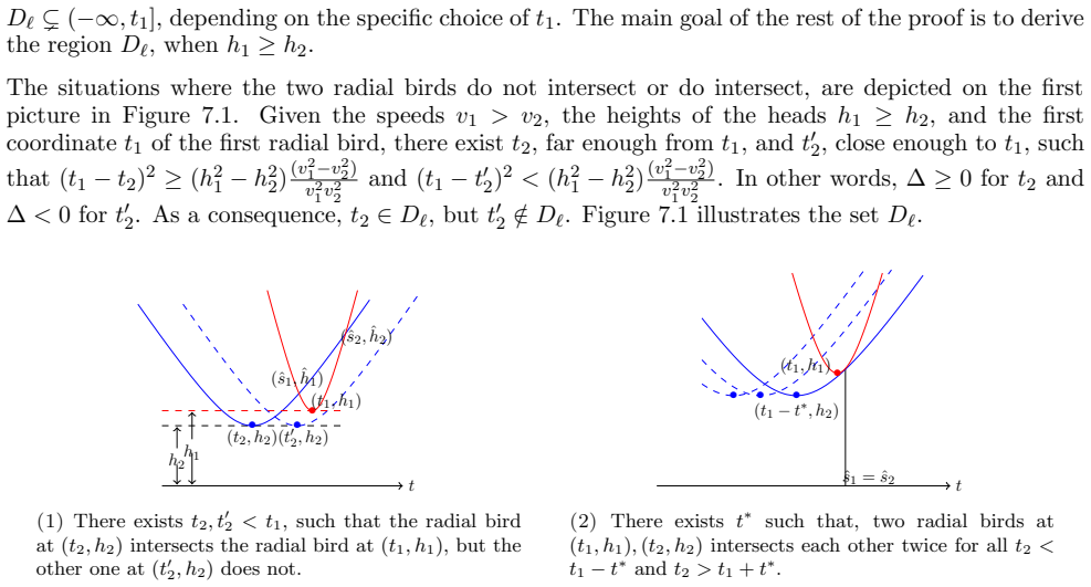
Figure 7.1. Figure 7.1: Criterion for intersections with v1 > v2, h1 > h2, fixed t1 but variable t2. In view of the last observation, given t1 and h1 ≥ h2, there exists a maximum value of t2 such that there is a unique intersection point of the two radial birds C1, C2, see Picture 7.12 of [PITH_FULL_IMAGE:figures/full_fig_p038_7_1.png] view at source ↗
Figure 7.2
Figure 7.2. Figure 7.2: Geometric interpretation of intersection criterion. where t ∗ = 1 v1v2 (h 2 − h 2 2 ) 1 2 (v 2 1 − v 2 2 ) 1 2 , as defined in (7.15). Any radial bird with head point on C˜ (t2,h2) and of type 1, intersects C 2 (t2,h2) exactly once, or equivalently, these two birds just touch each other. Here also, the set C˜ (t2,h2) is characterised by the curve given by t − t2 = ±t ∗ , i.e., (t − t2) 2 = 1 v 2 1 v 2 2 … view at source ↗
Figure 7.3
Figure 7.3. Figure 7.3: Under the bijection γ(t2,h2) , the point (ˆs, hˆ) is mapped to a point (t1, h1), such that the radial birds C 1 (t1,h1) , if it exists, touches C 2 (t2,h2) at (ˆs, hˆ). Note that for (ˆs, hˆ) and (ˆs1, hˆ 1) to represent two consecutive handovers, it is necessary that along with E s,v ˆ 1 hˆ ∪ E sˆ1,v1 hˆ1 , the extra region S, outside E s,v ˆ 1 hˆ ∪ E sˆ1,v1 hˆ1 , but below the hyperbola C˜ (t2,h2) betw… view at source ↗
Figure 7.4
Figure 7.4. Figure 7.4: The bird at (t1, h1) intersects the line L0 at level u, but the bird at (t2, h2) intersects the line L0 at level higher than u. Proof of part (ii). Without loss of generality, we prove the result for s = 0 also. We also assume 0 < t1 < t2, whereas the other case t2 < t1 < 0, can be proved similarly. The two more cases t2 < 0 < t1 and t1 < 0 < t2 can be derived from the cases 0 < t1 < t2 and t2 < t1 < 0, … view at source ↗
Figure 7.5
Figure 7.5. Figure 7.5: This is true because the radial bird of type 2 at ( [PITH_FULL_IMAGE:figures/full_fig_p041_7_5.png] view at source ↗
Figure 7.5
Figure 7.5. Figure 7.5: Scenario described in Lemma 7.13. by hˆ2 1 := v 2 1 s 2 1 − 2v 2 1 s1t1 + r 2 1 = v 2 2 s 2 1 − 2v 2 2 s1t2 + r 2 2 , hˆ2 2 := v 2 1 s 2 2 − 2v 2 1 s2t1 + r 2 1 = v 2 2 s 2 2 − 2v 2 2 s2t2 + r 2 2 . (7.21) Using the expressions of ˆs1, sˆ2 from (7.12) yields hˆ2 1 = v 2 1 [PITH_FULL_IMAGE:figures/full_fig_p042_7_5.png] view at source ↗
Figure 7.6
Figure 7.6. Figure 7.6: The handover distances ℓ1, ℓ2 are symmetric functions of t1 − t2, when v1 > v2. but the intersection distances remain the same. 7.1.7. Construction of the handover point process. In the following, we formally describe the construc￾tion of the handover point process V in the two-speed case. As seen before in the single-speed case, 42 [PITH_FULL_IMAGE:figures/full_fig_p042_7_6.png] view at source ↗
Figure 7.7
Figure 7.7. Figure 7.7: The labels at the intersections are the corresponding types, where the red and blue birds are of type 1 and 2 with speeds v1 > v2. In the following, we state the result about the time-stationarity of the handover point process V, which is inherited from the stationarity of the head point process H. Lemma 7.17 (Time-stationarity of V). In the two-speed case, the handover point process V is stationary with… view at source ↗
Figure 7.8
Figure 7.8. Figure 7.8: The mixed handovers seen in reverse time. We now show that Λ(1) 1,2 = Λ(2) 2,1 . Due to the bijection β (1) 1,2 in part (ii) of Lemma 7.18, one can associate each mixed intersection to the right-most head points or equivalently to the left-most head point. Let L (1) 1,2 be the point process on R made of the abscissas of the left-most head point corresponding to the handovers with the faster bird being on… view at source ↗
Figure 7.9
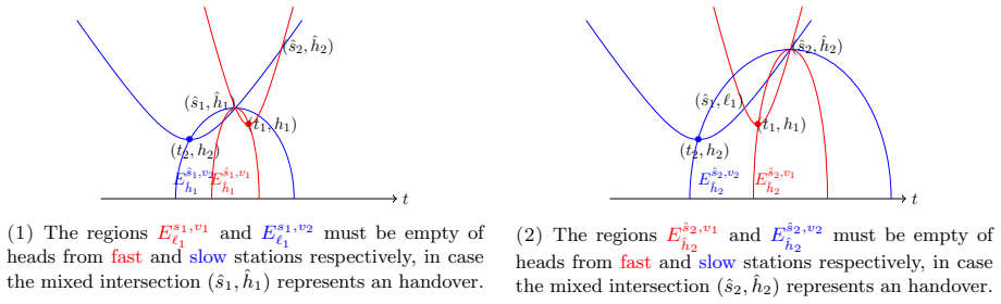
Figure 7.9. Figure 7.9: Mixed handovers due to first and second intersection of birds of two types. to (ˆsk, hˆ k) are given by, v 2 1 (t − sˆk) 2 + h 2 = hˆ2 k and v 2 2 (t − sˆk) 2 + h 2 = hˆ2 k (7.50) and the corresponding regions are E sˆk,v1 hˆ k and E sˆk,v2 hˆ k , respectively. For a point (ˆsk, hˆ k) to be a handover point, we need that the regions E sˆk,v1 hˆ k and E sˆk,v2 hˆ k be empty of points from H1 and H2 , resp… view at source ↗
Figure 7
Figure 7. Figure 7: ). Since [PITH_FULL_IMAGE:figures/full_fig_p049_7.png] view at source ↗
Figure 7.10
Figure 7.10. Figure 7.10: We consider (ˆs1, hˆ 1) = (ˆs (1) i,j , hˆ (1) i,j ), (ˆs2, hˆ 2) = (ˆs (2) i,j , hˆ (2) i,j ) for simplicity. The mixed intersec￾tion (ˆs1, hˆ 1) represents a handover if the regions E sˆ1,vi hˆ1 are empty of heads from Hi for all i ∈ [n]. The red and blue ellipses are for the speeds vj and vi , respectively and the green and black ones correspond to other speeds v ̸= vi , vj . Under the two-point Palm… view at source ↗
Figure 8.1
Figure 8.1. Figure 8.1: For (tn, hn) of type τn = 1 or 2 and for t ≥ tn, the pairs of upper half-ellipses  E t,v1 h1(t) , Et,v2 h1(t)  or  E t,v1 h2(t) , Et,v2 h2(t)  , respectively, benefit from the increasing wing property. 8.3.3. Palm distribution of inter-handover time. The following theorem determines the Laplace trans￾form of T, which is equal to T1(0), under the Palm probability distribution P 0 V in terms of the hea… view at source ↗
Figure 8.2
Figure 8.2. Figure 8.2: Transition diagram for all possible transitions among the handover types, where ∗ is used on two of the directed edges, to denote that the transition can happen in two possible ways. 66 [PITH_FULL_IMAGE:figures/full_fig_p066_8_2.png] view at source ↗
Figure 8.3
Figure 8.3. Figure 8.3: The only possibility for a future handover is hence (ˆs [PITH_FULL_IMAGE:figures/full_fig_p067_8_3.png] view at source ↗
Figure 8.3
Figure 8.3. Figure 8.3: The two cases in (8.44), i.e., the next handover can be given by a bird at (Tj , Hj ) = (t1, h1) of type 1 or 2, with (t1, h1) lying outside E s,v ˆ 1 hˆ or E s,v ˆ 2 hˆ , respectively. 68 [PITH_FULL_IMAGE:figures/full_fig_p068_8_3.png] view at source ↗
Figure 8.4
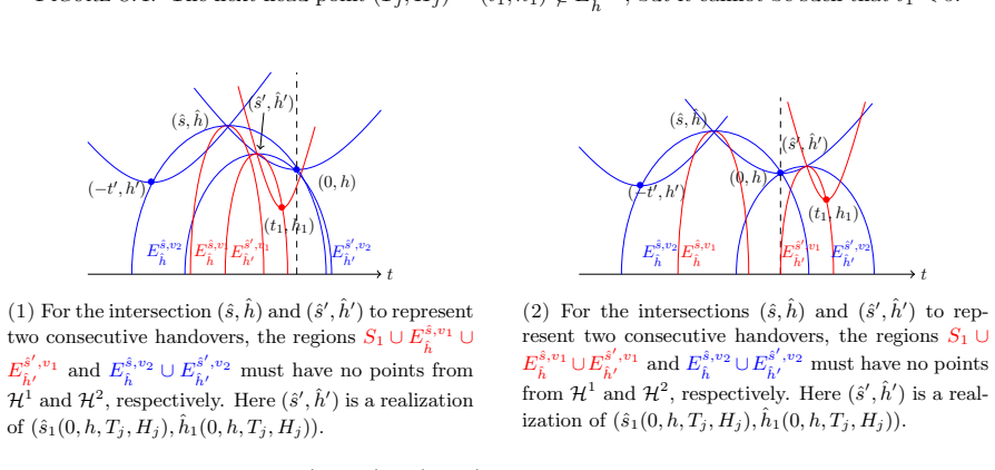
Figure 8.4. Figure 8.4: The next head point (Tj , Hj ) = (t1, h1) ∈/ E s,v ˆ 1 hˆ , but it cannot be such that t1 < sˆ. t • • (0, h) (−t ′ , h′) (ˆs ′ , hˆ′) (ˆs, hˆ) • (t1, h1) E s,v ˆ 2 hˆ E s,v ˆ 1 hˆ E sˆ ′ ,v2 E hˆ′ sˆ ′ ,v1 hˆ′ (1) For the intersection (ˆs, hˆ) and (ˆs ′ , hˆ′ ) to represent two consecutive handovers, the regions S1 ∪ E s,v ˆ 1 hˆ ∪ E sˆ ′ ,v1 hˆ′ and E s,v ˆ 2 hˆ ∪ E sˆ ′ ,v2 hˆ′ must have no points from… view at source ↗
Figure 8.5
Figure 8.5. Figure 8.5: The case where (Tj , Hj ) = (t1, h1) is of type 1. The two cases considered are, t1 < 0 and t1 ≥ 0, as in the first two terms in (8.52). 71 [PITH_FULL_IMAGE:figures/full_fig_p071_8_5.png] view at source ↗
Figure 8.6
Figure 8.6. Figure 8.6: The case where (t1, h1) is of type 2, with t1 ≥ 0, as in the last term in (8.52). For the intersections (ˆs, hˆ) and (ˆs ′ , hˆ′ ) to represent two consecutive handovers, the regions S2 ∪ E s,v ˆ 1 hˆ ∪ E sˆ ′ ,v1 hˆ′ and E s,v ˆ 2 hˆ ∪ E sˆ ′ ,v2 hˆ′ must have no points from H1 and H2 , respectively. Here (ˆs ′ , hˆ′ ) is a realization of (ˆs(0, h, Tj , Hj ), hˆ(0, h, Tj , Hj )). 72 [PITH_FULL_IMAGE:fi… view at source ↗
Figure 8.7
Figure 8.7. Figure 8.7: Thus we have T1(ˆs1) := ˆs(0, h, Tj , Hj ). For this intersection to give the next handover immediately after time ˆs1, the extra region S t∈[ˆs1,sˆ(0,h,Tj ,Hj )] E t,vl hˆt \ E sˆ1,vl hˆ 1 o , beyond E sˆ1,vl hˆ 1 , must have no point of Hl for l = 1, 2, where hˆ t = (v 2 1 t 2 + h 2 ) 1 2 . The union is due to Definition 8.13 and to the fact that the sets in the union potentially lack monotonicity. S… view at source ↗
Figure 8.7
Figure 8.7. Figure 8.7: The cases corresponding to the first and second term in (8.62), when the head point (Tj , Hj ) = (t1, h1) is of type 1 and 2, respectively. t • (−t ′ , h′) • (0, h) (ˆs1, hˆ 1) (ˆs2, hˆ 2) E sˆ1,v2 hˆ 1 E sˆ1,v1 hˆ 1 E sˆ2,v2 hˆ 2 E sˆ2,v1 hˆ 2 [PITH_FULL_IMAGE:figures/full_fig_p076_8_7.png] view at source ↗
Figure 8.8
Figure 8.8. Figure 8.8: The case corresponding to the last term in (8.63). For the intersections (ˆs1, hˆ 1) and (ˆs2, hˆ 2) to represent two consecutive handovers, the regions E sˆ1,v1 hˆ1 ∪ E sˆ2,v1 hˆ2 and E sˆ1,v2 hˆ1 ∪ E sˆ2,v2 hˆ2 must have no points from H1 and H2 , respectively. Thus, based on the last arguments, we write the inner expectation in (8.61), as the following sum of three terms: 76 [PITH_FULL_IMAGE:figures/… view at source ↗
Figure 8.9
Figure 8.9. Figure 8.9: For the two intersection points to represent handovers, we must have no point of [PITH_FULL_IMAGE:figures/full_fig_p079_8_9.png] view at source ↗
Figure 8.10
Figure 8.10. Figure 8.10: Thus we have T1(ˆs1) := ˆs2(−t ′ , h′ , Tj , Hj ). The last intersection to give a handover, the extra region S t∈[ˆs1,sˆ2(−t ′ ,h′ ,Tj ,Hj )] E t,vl hˆt \ E sˆ1,vl hˆ 1 o must have not points of Hl for l = 1, 2. The union is due to Definition 8.13 and the fact that individual sets in the union potentially lack monotonicity. t (−t • ′ , h′) • (0, h) • (t1, h1) (ˆs1, hˆ 1) (ˆs2, hˆ 2) (˜s, h˜) E sˆ1,v2… view at source ↗
Figure 8.11
Figure 8.11. Figure 8.11: The case corresponding to the last term in (8.80). For the intersections (ˆs1, hˆ 1) and (ˆs2, hˆ 2) to represent two consecutive handovers, the regions E sˆ1,v1 hˆ1 ∪ E sˆ2,v1 hˆ2 and E sˆ1,v2 hˆ1 ∪ E sˆ2,v2 hˆ2 must have no points from H1 and H2 , respectively. The point (Tj , Hj ) must lie in the region R1(h, t′ , h′ ) ⊂ [−t ′ , ∞) × R + \ E sˆ1,v1 hˆ 1 be the region defined as R1(h, t′ , h′ ) :=  (… view at source ↗
Figure 8.12
Figure 8.12. Figure 8.12: Case 1 and Case 2, when the head point (Tj , Hj ) = (t1, h1) is of type 1 or 2, respectively. Using Remark 7.10 for the first two terms in (8.89) for l = 1, we have [ t∈[ˆs2,sˆ1(0,h,Tj ,Hj )] E t,v1 hˆt ∪ E sˆ2,v1 hˆ 2 = E sˆ2,v1 hˆ 2 ∪ S1 ∪ E sˆ1(0,h,Tj ,Hj ),v1 hˆ 1(0,h,Tj ,Hj ) , where hˆ t = (v 2 2 t 2 + h 2 ) 1 2 and S1 is the region outside E sˆ2,v1 hˆ 2 ∪ E sˆ1(0,h,Tj ,Hj ),v1 hˆ 1(0,h,Tj ,Hj ) ,… view at source ↗
Figure 5
Figure 5. Figure 5: ) is [PITH_FULL_IMAGE:figures/full_fig_p106_5.png] view at source ↗
read the original abstract

Consider a dynamical network model featuring mobile stations on the Euclidean plane. The initial locations of the stations are given by a homogeneous Poisson point process. The stations are all moving at a constant speed and in a random direction. Consider fixed users located in the Euclidean plane, which are served by the mobile stations. Each user stays connected to the nearest station at any given point of time. Since the stations are moving, a user disconnects and connects with different stations over time, by always selecting which ever station is the closest. This gives rise to a dynamical version of the Poisson-Voronoi tessellation. The focus of this paper is on the sequence of ``handover'' events of a typical user, which are the epochs when its association changes. This defines a point process on the time-axis, the ``handover point process''. We show that this point process is stationary and we determine its main properties, in particular its intensity and the joint distribution of its inter-event times. We also analyze the handover Palm distributions of several variables of practical interest. This includes the distance to the closest mobile stations and the point process of all other mobile stations at handover epochs. The analysis is conducted both in the single-speed and in the multi-speed scenarios. It leads to the identification of the three dimensional state variables that ``Markovize'' the association dynamics. The analysis is based on a specific system of non compact particles. The motivations are in the modeling of low or medium orbit satellite wireless communication networks. The model studied here is a planar ``caricature'' of this problem, which is initially defined on the sphere.

Editorial analysis

A structured set of objections, weighed in public.

Desk editor's note, referee report, simulated authors' rebuttal, and a circularity audit. Tearing a paper down is the easy half of reading it; the pith above is the substance, this is the friction.

Referee Report

1 major / 2 minor

Summary. The paper studies a dynamical Poisson-Voronoi tessellation generated by mobile stations whose initial positions form a homogeneous Poisson point process on the Euclidean plane, each moving at constant speed in a random direction. For a typical fixed user, the sequence of handover events (times when the serving station changes) defines a point process on the time axis. The authors establish that this handover point process is stationary, compute its intensity and the joint distribution of inter-event times, and examine the Palm distributions at handover epochs for quantities such as distance to the nearest station and the configuration of other stations. The analysis covers both single-speed and multi-speed regimes and identifies a three-dimensional Markov state (distance to nearest station, relative velocity components, and angular variable) that governs the association dynamics.

Significance. If the results hold, the paper supplies a rigorous stochastic-geometry treatment of handover processes in a mobile Poisson-Voronoi setting that serves as a planar caricature for low- or medium-orbit satellite networks. The explicit intensity formula, joint inter-event distribution, and Markovian reduction to a three-dimensional state provide concrete, computable tools for performance analysis. The construction rests directly on the time-homogeneous Poisson point process and i.i.d. constant-velocity motions, with no evident circularity or hidden compactness assumptions.

major comments (1)
  1. The reduction to the three-dimensional Markov state is load-bearing for the derivation of the intensity and inter-event distributions; the manuscript should explicitly verify that the generator of this state (distance, relative velocity components, angular variable) is sufficient to determine the future evolution of the association process in both the single-speed and multi-speed cases.
minor comments (2)
  1. Notation for the multi-speed regime should be introduced with a short comparison table or paragraph distinguishing it from the single-speed case to improve readability.
  2. The term 'non compact particles' appearing in the abstract and introduction would benefit from a one-sentence clarification for readers outside the immediate subfield.

Simulated Author's Rebuttal

1 responses · 0 unresolved

We thank the referee for the positive evaluation and the recommendation of minor revision. We address the single major comment below and will incorporate the requested clarification.

read point-by-point responses
  1. Referee: The reduction to the three-dimensional Markov state is load-bearing for the derivation of the intensity and inter-event distributions; the manuscript should explicitly verify that the generator of this state (distance to nearest station, relative velocity components, and angular variable) is sufficient to determine the future evolution of the association process in both the single-speed and multi-speed cases.

    Authors: We agree that an explicit verification of the Markov property via the infinitesimal generator would strengthen the exposition. Although the manuscript already identifies the three-dimensional state (distance to nearest station, relative velocity components, and angular variable) that Markovizes the association dynamics, we will add a dedicated paragraph deriving the generator and confirming that it fully governs the future evolution of the handover process. This verification will rely on the lack of memory in the underlying Poisson point process and the deterministic constant-velocity motions, and will be provided separately for the single-speed and multi-speed regimes. revision: yes

Circularity Check

0 steps flagged

No significant circularity; derivation self-contained from PPP and motion primitives

full rationale

The paper establishes stationarity of the handover point process and computes its intensity plus joint inter-event distributions from the given homogeneous Poisson point process of initial station locations together with i.i.d. constant-velocity random directions. The three-dimensional Markov state (nearest-station distance, relative velocity components, angular variable) is obtained directly by reduction of these primitives; the generator then yields the Palm distributions and intensity without any fitted parameters, self-referential definitions, or load-bearing self-citations. Both single-speed and multi-speed regimes follow from the same construction, which remains externally verifiable against the stated model assumptions.

Axiom & Free-Parameter Ledger

2 free parameters · 2 axioms · 0 invented entities

The central claim relies on standard assumptions from point process theory and motion models, with no new entities postulated.

free parameters (2)
  • Poisson intensity λ
    The density of the initial point process, a standard model parameter.
  • Speed(s) v
    The constant speed of motion, possibly varying in multi-speed case.
axioms (2)
  • domain assumption Initial locations form a homogeneous Poisson point process on the plane.
    Fundamental assumption for the model as stated in the abstract.
  • domain assumption Each station moves with constant velocity in a uniformly random direction.
    Key modeling choice for the dynamics.

pith-pipeline@v0.9.0 · 5826 in / 1442 out tokens · 81611 ms · 2026-05-21T17:51:16.935338+00:00 · methodology

discussion (0)

Sign in with ORCID, Apple, or X to comment. Anyone can read and Pith papers without signing in.

Lean theorems connected to this paper

Citations machine-checked in the Pith Canon. Every link opens the source theorem in the public Lean library.

What do these tags mean?
matches
The paper's claim is directly supported by a theorem in the formal canon.
supports
The theorem supports part of the paper's argument, but the paper may add assumptions or extra steps.
extends
The paper goes beyond the formal theorem; the theorem is a base layer rather than the whole result.
uses
The paper appears to rely on the theorem as machinery.
contradicts
The paper's claim conflicts with a theorem or certificate in the canon.
unclear
Pith found a possible connection, but the passage is too broad, indirect, or ambiguous to say the theorem truly supports the claim.

Forward citations

Cited by 1 Pith paper

Reviewed papers in the Pith corpus that reference this work. Sorted by Pith novelty score.

  1. Seasonal Statistics of Shannon Capacity in a Dynamical Poisson-Voronoi Cellular Network

    math.PR 2026-05 unverdicted novelty 5.0

    Analysis of Shannon capacity statistics at handover, proximity, and interference epochs in a dynamical Poisson-Voronoi network with an analogy to seasonal fluctuations in signal quality.

Reference graph

Works this paper leans on

26 extracted references · 26 canonical work pages · cited by 1 Pith paper

  1. [1]

    Albers and T

    G. Albers and T. Roos. Voronoi diagrams of moving points in higher dimensional spaces.Lecture Notes in Computer Science, vol. 621. (Proceedings of the Third Scandinavian Workshop on Algorithm Theory, SWAT 1992. Springer, Berlin, Heidelberg

  2. [2]

    G. Albers. Three-Dimensional Dynamic Voronoi Diagrams. Diploma thesis, University of W¨ urzburg, 1991

  3. [3]

    Baccelli, B

    F. Baccelli, B. B laszczyszyn and M. Karray. Random Measures, Point Processes, Stochastic Geometry.Inria, 2020. https://hal.inria.fr/hal-02460214

  4. [4]

    Baccelli and P

    F. Baccelli and P. Br´ emaud. Elements of Queueing Theory: Palm Martingale Calculus and Stochastic Recurrences. Springer Berlin, Heidelberg, 2003

  5. [5]

    Baccelli and C

    F. Baccelli and C. S. Choi. A Novel Analytical Model for LEO Satellite Constellations Leveraging Cox Point Processes, IEEE Transactions on Communications, 73(4):2265–2279, 2025

  6. [6]

    Baccelli, M

    F. Baccelli, M. Klein, M. Lebourges and S. Zuyev. Stochastic geometry and architecture of communication networks. Telecommunication Systems, 7:209–227, 1997

  7. [7]

    Baccelli, P

    F. Baccelli, P. Madadi and G. de Veciana. Shared Rate Process for Mobile Users in Poisson Networks and Applications. IEEE Transactions on Information Theory, 64(3):2121–2141, 2018

  8. [8]

    Baccelli and S

    F. Baccelli and S. Zuyev. Stochastic geometry models of mobile communication networks. InFrontiers in Queueing: Models and Applications in Science and Engineering, ed. J. Dshalalow, Chapter 8:227–243. CRC Press, 1996

  9. [9]

    Baccelli and S

    F. Baccelli and S. Zuyev. Poisson-Voronoi Spanning Trees with Applications to the Optimization of Communication Networks. Oper. Res., 47(4):619–631, 1999

  10. [10]

    A. Beutel. Interactive Voronoi Diagram Generator with WebGL.https://alexbeutel.com/webgl/voronoi.html, 2012

  11. [11]

    E. N. Gilbert. Random subdivisions of space into chrystals.Adv. Appl. Prob., 33:958–972, 1962

  12. [12]

    Gowda, D

    I. Gowda, D. Kirkpatrick, D. Lee and A. Naamad. Dynamic Voronoi diagrams.IEEE Transactions on Information Theory, 29(5):724–731, 1983

  13. [13]

    Heinrich

    L. Heinrich. Contact and chord length distribution of a stationary Voronoi tessellation.Adv. Appl. Prob., 30:603–618, 1998

  14. [14]

    J. F. C. Kingman. Poisson Processes,Oxford University Press, USA, 1993

  15. [15]

    J. Mecke. Formulas for stationary planar fiber processes III—intersection with fiber systems. Math. Oper. Statist. 12:201–210, 1981

  16. [16]

    R. E. Miles. Sectional Voronoi tessellation.Revista de la Uni´ on Matem´ atica Argentina, 29:310–327, 1984

  17. [17]

    M¨ oller

    J. M¨ oller. Random tessellations inRd. Adv. Appl. Probab., 21:37–73, 1989

  18. [18]

    T. Roos. Voronoi diagrams over dynamic scenes.Discrete Appl. Math., 43(3):243–259, 1993

  19. [19]

    T. Roos. Dynamic Voronoi diagrams. Ph.D. Thesis, University of W¨ urzburg, 1991

  20. [20]

    L. Muche. Contact and Chord Length Distribution Functions of the Poisson-Voronoi Tessellation in High Dimensions. Adv. Appl. Probab.42(1):48–68, 2010

  21. [21]

    Muche and D

    L. Muche and D. Stoyan. Contact and chord length distributions of the Poisson Voronoi tessellation.J. Appl. Prob., 29:467–471, 1992

  22. [22]

    Okabe, B

    A. Okabe, B. Boots, K. Sugihara and S. N. Chiu. Spatial tessellations: Concepts and applications of Voronoi diagrams. John Wiley and Sons, second edition, 2000

  23. [23]

    Okati, T

    N. Okati, T. Riihonen, D. Korpi, I. Angervuori and R. Wichman. Downlink Coverage and Rate Analysis of Low Earth Orbit Satellite Constellations Using Stochastic Geometry.IEEE Transactions on Communications, 68(8):5120–5134, 2020

  24. [24]

    N. Okati. Modeling and Analysis of Massive Low Earth Orbit Communication Networks. Ph.D. Thesis, Tempere University:https://trepo.tuni.fi/handle/10024/146346, 2023

  25. [25]

    C. Palm. Intensit¨ atsschwankungen im fernsprechverkehr.Ericsson Technics, 1943

  26. [26]

    D. Stoyan. Comparison Methods for Queues and other Stochastic Models.J. Wiley and Sons, Chichester, 1983. (FB)MATHNET, INRIA Paris, 48 Rue Barrault, 75013 Paris, France, and INFRES, T ´el´ecom Paris, 19, place Marguerite Perey, 91123 Palaiseau, France Email address:francois.baccelli@inria.fr (SKJ)INFRES, T ´el´ecom Paris, 19, place Marguerite Perey, 91123...