Boundary treatment algorithms for meshfree RANS turbulence modeling
Pith reviewed 2026-05-16 13:24 UTC · model grok-4.3
The pith
The nearest-band neighbor method enables stable wall-function enforcement in meshfree simulations of turbulent flows over curved surfaces.
A machine-rendered reading of the paper's core claim, the machinery that carries it, and where it could break.
Core claim
The nearest-band neighbor method, which enforces wall functions on a band of interior points rather than isolated closest neighbors, supplies a stable and flexible treatment that outperforms both the baseline closest-neighbor scheme and the shifted-boundary scheme on practical curved geometries such as the NACA 0012 airfoil.
What carries the argument
The nearest-band neighbor (NBN) method that selects a band of interior points to enforce wall functions, thereby preserving uniform distance sampling in scattered, possibly moving point clouds.
If this is right
- Meshfree RANS modeling becomes practical for engineering geometries once the nearest-band neighbor treatment is used.
- The shifted-boundary method delivers perfectly smooth y-plus distributions and high stability on flat plates.
- All three common closures (Spalart-Allmaras, k-ε, k-ω) produce consistent results when paired with the nearest-band neighbor scheme.
- The method avoids the numerical diffusion and early separation observed when shifted-boundary points are used on curved surfaces.
Where Pith is reading between the lines
- The same band-selection idea could be applied directly to other Lagrangian meshfree schemes without requiring new turbulence-model development.
- Correcting normal vectors inside the shifted-boundary step might remove the curvature-related errors and make that method viable for airfoils as well.
- Because the approach works with existing turbulence closures, it can be inserted into existing meshfree codes with only local changes to the boundary stencil.
Load-bearing premise
Point distributions and normal vectors remain free of excessive clustering or uncorrected shifting that would distort wall-distance enforcement on curved surfaces under adverse pressure gradients.
What would settle it
Premature flow separation or markedly increased numerical diffusion appearing in NBN results on the NACA 0012 airfoil at Reynolds numbers of order 10^6, matching the shortcomings already seen with the shifted-boundary method.
Figures


read the original abstract
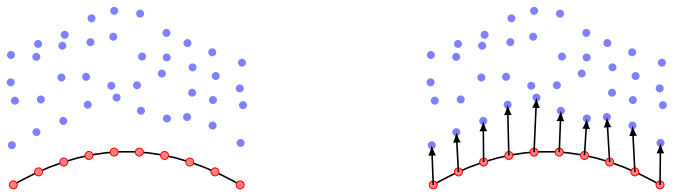
In this paper, we propose improved wall-treatment strategies for meshfree methods applied to turbulent flows. The goal is to enhance wall-function handling in simulations of high-Reynolds-number turbulent flows and to understand the performance of turbulence models within these frameworks. While wall-function techniques are well established for mesh-based methods, their implementation in meshfree methods faces unique challenges. The main difficulties arise from scattered point distributions and dynamic point movement in Lagrangian frameworks. To address these issues, we evaluate a baseline closest-neighbor approach alongside two novel techniques: the nearest-band neighbor (NBN) method and the shifted boundary (SB) method. The NBN method enforces wall functions on a band of interior points, helping to maintain uniform point selection. On the other hand, the SB method virtually moves boundary points to a fixed wall-normal distance, eliminating the spatial noise associated with point movement. We evaluate these methods using turbulence closures: Spalart--Allmaras, $k-\varepsilon$, and $k-\omega$ turbulence models. These methods are validated on 1D Couette flow, a turbulent flat plate, and a 3D NACA 0012 airfoil at high Reynolds numbers. Results demonstrate that both novel methods outperform the standard closest-neighbor approach on flat geometries. For flat plates, the SB method provides stability and perfectly smooth $y^+$ distributions. However, when applied to a curved NACA 0012 profile, the NBN method proves to be robust and flexible. In contrast, the SB method exhibits setbacks in numerical diffusion and premature flow separation on curved geometries. This is due to uncorrected normal-vector shifting and adverse pressure gradients. This work establishes the NBN method as a reliable, robust foundation for simulating turbulent flows over practical geometries using meshfree methods.
Editorial analysis
A structured set of objections, weighed in public.
Referee Report
Summary. The manuscript proposes two novel boundary treatment algorithms—nearest-band neighbor (NBN) and shifted boundary (SB)—for meshfree RANS turbulence modeling to improve wall-function handling in high-Re flows. These are evaluated against a baseline closest-neighbor approach using Spalart–Allmaras, k–ε, and k–ω closures on 1D Couette flow, a turbulent flat plate, and a 3D NACA 0012 airfoil. The central claims are that both new methods outperform the baseline on flat geometries, SB yields perfectly smooth y+ on flat plates, and NBN is robust and flexible on the curved airfoil while SB suffers premature separation from uncorrected normal-vector shifting under adverse pressure gradients.
Significance. If the quantitative validation gaps were closed, the work could supply practical boundary treatments for meshfree methods applied to turbulent flows over realistic geometries, directly addressing scattered-point and Lagrangian-movement difficulties. The multi-model, multi-geometry test suite is a constructive element, yet the current absence of absolute error metrics against experiments or established mesh-based RANS solutions limits immediate utility for the community.
major comments (2)
- [Abstract] Abstract: the statement that both novel methods outperform the baseline on flat geometries is unsupported by any quantitative metrics (e.g., skin-friction profiles, velocity errors, or y+ statistics) or error bars; only qualitative validation statements are supplied.
- [Abstract] Abstract (NACA 0012 results): the claim that NBN constitutes a reliable, robust foundation for practical curved geometries rests solely on relative improvement over closest-neighbor and SB; no absolute accuracy metrics (Cd, Cl, Cf distributions, or y+ profiles) benchmarked against experimental data or mesh-based RANS solutions at the same Re and angle of attack are reported, leaving the central claim without direct verification.
minor comments (2)
- The abstract refers to 'high Reynolds numbers' without stating the precise values employed for the flat-plate and airfoil cases.
- A summary table collating quantitative performance indicators (drag, lift, separation location, etc.) across all three test cases and all three turbulence models would improve readability and allow direct comparison.
Simulated Author's Rebuttal
We thank the referee for the constructive and detailed review of our manuscript. We address each major comment point by point below, indicating the revisions we will make to strengthen the presentation of our results.
read point-by-point responses
-
Referee: [Abstract] Abstract: the statement that both novel methods outperform the baseline on flat geometries is unsupported by any quantitative metrics (e.g., skin-friction profiles, velocity errors, or y+ statistics) or error bars; only qualitative validation statements are supplied.
Authors: We agree that the abstract would benefit from explicit quantitative support. The full manuscript contains quantitative comparisons via skin-friction coefficient distributions, velocity profiles, and y+ statistics for the flat-plate cases that demonstrate the improvements. We will revise the abstract to include specific quantitative statements drawn from these results, such as the reduction in skin-friction deviation from reference values and the uniformity of y+ distributions. revision: yes
-
Referee: [Abstract] Abstract (NACA 0012 results): the claim that NBN constitutes a reliable, robust foundation for practical curved geometries rests solely on relative improvement over closest-neighbor and SB; no absolute accuracy metrics (Cd, Cl, Cf distributions, or y+ profiles) benchmarked against experimental data or mesh-based RANS solutions at the same Re and angle of attack are reported, leaving the central claim without direct verification.
Authors: The central objective of the work is to compare boundary-treatment algorithms within the meshfree RANS framework. For the NACA 0012 airfoil we demonstrate that NBN avoids the premature separation and excessive numerical diffusion exhibited by SB under adverse pressure gradients while remaining more stable than the closest-neighbor approach. We acknowledge that absolute metrics against experiments or mesh-based RANS are not included. We will revise the abstract to qualify the robustness claim as relative to the other meshfree treatments and add a brief discussion of this limitation in the conclusions. revision: partial
- Absolute accuracy metrics (Cd, Cl, Cf distributions, or y+ profiles) for the NACA 0012 airfoil benchmarked against experimental data or established mesh-based RANS solutions at matching Re and angle of attack are not available in the present study.
Circularity Check
No circularity: methods validated on independent external benchmarks
full rationale
The paper proposes NBN and SB wall-treatment algorithms for meshfree RANS, then evaluates them comparatively against the baseline closest-neighbor method on three standard external benchmark flows (1D Couette, turbulent flat plate, 3D NACA 0012 at high Re). No equations, parameters, or central claims are shown to reduce by construction to fitted inputs, self-definitions, or load-bearing self-citations; performance statements rest on relative numerical outcomes against known reference solutions rather than internal renaming or ansatz smuggling. The derivation chain is therefore self-contained against external data.
Axiom & Free-Parameter Ledger
axioms (1)
- domain assumption Standard RANS turbulence model assumptions (Spalart-Allmaras, k-ε, k-ω) hold for the tested high-Re flows
Reference graph
Works this paper leans on
-
[1]
M. Antuono et al. “Smoothed particle hydrodynamics method from a large eddy simulation perspective. Generalization to a quasi-Lagrangian model” . en. In: Physics of Fluids 33.1 (2021), p. 015102
work page 2021
-
[2]
Large eddy simulation and a simple wall model for turbulent flow calculation by a particle method
Jun Arai, Seiichi Koshizuka, and Koji Murozono. “Large eddy simulation and a simple wall model for turbulent flow calculation by a particle method” . en. In: International Journal for Numerical Methods in Fluids 71.6 (2013), pp. 772–787
work page 2013
-
[3]
Extensions of the Spalart–Allmaras turbulence model to account for wall roughness
B. Aupoix and P.R. Spalart. “Extensions of the Spalart–Allmaras turbulence model to account for wall roughness” . en. In: International Journal of Heat and Fluid Flow 24.4 (2003), pp. 454–462
work page 2003
-
[4]
Tingting Bao et al. “Smoothed particle hydrodynamics with k - ϵ closure for simulating wall-bounded turbulent flows at medium and high Reynolds numbers” . en. In: Physics of Fluids 35.8 (2023), p. 085114
work page 2023
-
[5]
Meshless methods: An overview and recent developments
T. Belytschko et al. “Meshless methods: An overview and recent developments” . en. In: Computer Methods in Applied Mechanics and Engineering 139.1-4 (1996), pp. 3–47
work page 1996
-
[6]
J. Boussinesq. Essai sur la théorie des eaux courantes. Mémoires présentés par divers savants à l’Académie des sciences de l’Institut national de France. Impr. nationale, 1877
-
[7]
On the Wall Boundary Condition for Turbulence Models
Jonas Bredberg. On the Wall Boundary Condition for Turbulence Models. 2000
work page 2000
-
[8]
Accurate Projection Methods for the Incompressible Navier–Stokes Equations
David L. Brown, Ricardo Cortez, and Michael L. Minion. “Accurate Projection Methods for the Incompressible Navier–Stokes Equations” . In: Journal of Computational Physics 168.2 (2001), pp. 464–499
work page 2001
-
[9]
Meshfree Methods: Progress Made after 20 Years
Jiun-Shyan Chen, Michael Hillman, and Sheng-Wei Chi. “Meshfree Methods: Progress Made after 20 Years” . en. In: Journal of Engineering Mechanics 143.4 (2017), p. 04017001. 26
work page 2017
-
[10]
Predictions of Channel and Boundary-Layer Flows with a Low- Reynolds-Number Turbulence Model
Kuei-Yuan Chien. “Predictions of Channel and Boundary-Layer Flows with a Low- Reynolds-Number Turbulence Model” . en. In: AIAA Journal 20.1 (1982), pp. 33–38
work page 1982
-
[11]
Numerical solution of the Navier-Stokes equations
Alexandre Joel Chorin. “Numerical solution of the Navier-Stokes equations” . In: Mathematics of computation 22.104 (1968), pp. 745–762
work page 1968
-
[12]
The law of the wake in the turbulent boundary layer
Donald Coles. “The law of the wake in the turbulent boundary layer” . en. In: Journal of Fluid Mechanics 1.2 (1956), pp. 191–226
work page 1956
-
[13]
Progress in the generalization of wall-function treatments
T.J. Craft et al. “Progress in the generalization of wall-function treatments” . en. In: International Journal of Heat and Fluid Flow 23.2 (2002). Publisher: Elsevier BV, pp. 148–160
work page 2002
-
[14]
Finite pointset method for simulation of the liquid - liquid flow field in an extractor
Christian Drumm et al. “Finite pointset method for simulation of the liquid - liquid flow field in an extractor” . In: Computers & Chemical Engineering 32.12 (2008), pp. 2946– 2957
work page 2008
- [15]
-
[16]
On the state-of-the-art of particle methods for coastal and ocean engineering
Hitoshi Gotoh and Abbas Khayyer. “On the state-of-the-art of particle methods for coastal and ocean engineering” . en. In: Coastal Engineering Journal 60.1 (2018), pp. 79– 103
work page 2018
-
[17]
Drag and Turbulent Boundary Layer of Flat Plates at Low Reynolds Numbers
Paul S. Granville. “Drag and Turbulent Boundary Layer of Flat Plates at Low Reynolds Numbers” . en. In: Journal of Ship Research 21.01 (1977), pp. 30–39
work page 1977
-
[18]
An Overview of Meshfree Collocation Methods
Tomas Halada et al. “An Overview of Meshfree Collocation Methods” . In: arXiv preprint arXiv:2509.20056 (2025)
-
[19]
A multi-phase SPH method for macroscopic and mesoscopic flows
X.Y. Hu and N.A. Adams. “A multi-phase SPH method for macroscopic and mesoscopic flows” . en. In: Journal of Computational Physics 213.2 (2006), pp. 844–861
work page 2006
-
[20]
Finite Pointset Method for the Simulation of a Vehicle Travelling Through a Body of Water
Anthony Jefferies et al. “Finite Pointset Method for the Simulation of a Vehicle Travelling Through a Body of Water” . In: Meshfree Methods for Partial Differential Equations VII. Ed. by Michael Griebel and Alexander Marc Schweitzer. Cham: Springer International Publishing, 2015, pp. 205–221
work page 2015
-
[21]
Temperature and concentration profiles in fully turbulent boundary layers
B.A. Kader. “Temperature and concentration profiles in fully turbulent boundary layers” . en. In: International Journal of Heat and Mass Transfer 24.9 (1981), pp. 1541–1544
work page 1981
-
[22]
Near-wall behavior of RANS turbulence models and implications for wall functions
Georgi Kalitzin et al. “Near-wall behavior of RANS turbulence models and implications for wall functions” . en. In: Journal of Computational Physics 204.1 (2005), pp. 265–291
work page 2005
-
[23]
Meshfree numerical scheme for time dependent problems in fluid and continuum mechanics
Joerg Kuhnert. “Meshfree numerical scheme for time dependent problems in fluid and continuum mechanics” . In: Advances in PDE Modeling and Computation. Ed. by S. Sundar. New Delhi: Anne Books, 2014, pp. 119–136
work page 2014
-
[24]
C.L. Ladson et al. Effects of Independent Variation of Mach and Reynolds Numbers on the Low-speed Aerodynamic Characteristics of the NACA 0012 Airfoil Section. NASA technical memorandum. National Aeronautics, Space Administration, Scientific, and Technical Information Division, 1988
work page 1988
-
[25]
The numerical computation of turbulent flows
B.E. Launder and D.B. Spalding. “The numerical computation of turbulent flows” . en. In: Computer Methods in Applied Mechanics and Engineering 3.2 (1974), pp. 269–289
work page 1974
-
[26]
The finite difference method at arbitrary irregular grids and its application in applied mechanics
T. Liszka and J. Orkisz. “The finite difference method at arbitrary irregular grids and its application in applied mechanics” . en. In: Computers & Structures 11.1-2 (1980), pp. 83–95
work page 1980
-
[27]
Gui-Rong Liu and Y. T. Gu. An introduction to Meshfree methods and their programming. eng. Dordrecht: Springer, 2010
work page 2010
-
[28]
An advancing front point generation technique
Rainald Löhner and Eugenio Oñate. “An advancing front point generation technique” . en. In: Communications in Numerical Methods in Engineering 14.12 (1998), pp. 1097–1108
work page 1998
-
[29]
Towards SPH simulations of cavitating flows with an EoSB cavitation model
Hong-Guan Lyu et al. “Towards SPH simulations of cavitating flows with an EoSB cavitation model” . en. In: Acta Mechanica Sinica 39.2 (2023), p. 722158
work page 2023
-
[30]
Wall-bounded turbulent flows at high Reynolds numbers: Recent advances and key issues
I. Marusic et al. “Wall-bounded turbulent flows at high Reynolds numbers: Recent advances and key issues” . en. In: Physics of Fluids 22.6 (2010), p. 065103
work page 2010
-
[31]
Takeharu Matsuda and Satoshi Ii. A least-squares meshfree method for the incompressible Navier-Stokes equations: A satisfactory solenoidal velocity field via a staggered-variable arrangement. Version Number: 1. 2025. 27
work page 2025
-
[32]
DNS and LES of 3-D wall-bounded turbulence using Smoothed Particle Hydrodynamics
A. Mayrhofer et al. “DNS and LES of 3-D wall-bounded turbulence using Smoothed Particle Hydrodynamics” . en. In: Computers & Fluids 115 (2015), pp. 86–97
work page 2015
-
[33]
Two-equation eddy-viscosity turbulence models for engineering applications
F. R. Menter. “Two-equation eddy-viscosity turbulence models for engineering applications” . en. In: AIAA Journal 32.8 (1994), pp. 1598–1605
work page 1994
-
[34]
Large eddy simulation within the smoothed particle hydrodynamics: Applications to multiphase flows
Domenico Davide Meringolo et al. “Large eddy simulation within the smoothed particle hydrodynamics: Applications to multiphase flows” . en. In: Physics of Fluids 35.6 (2023), p. 063312
work page 2023
-
[35]
A meshfree generalized finite difference method for solution mining processes
Isabel Michel et al. “A meshfree generalized finite difference method for solution mining processes” . In: Computational Particle Mechanics 8.3 (2021), pp. 561–574
work page 2021
-
[36]
Smoothed Particle Hydrodynamics and Its Diverse Applications
J.J. Monaghan. “Smoothed Particle Hydrodynamics and Its Diverse Applications” . en. In: Annual Review of Fluid Mechanics 44.1 (2012), pp. 323–346
work page 2012
-
[37]
Numerical Simulation of Turbulent Flows Using a Least Squares Based Meshless Method
M. Naghian, M. Lashkarbolok, and E. Jabbari. “Numerical Simulation of Turbulent Flows Using a Least Squares Based Meshless Method” . en. In: International Journal of Civil Engineering 15.1 (2017), pp. 77–87
work page 2017
-
[38]
Wall-layer boundary condition method for laminar and turbulent flows in weakly-compressible SPH
Akihiko Nakayama, Xin Yan Lye, and Khai Ching Ng. “Wall-layer boundary condition method for laminar and turbulent flows in weakly-compressible SPH” . en. In: European Journal of Mechanics - B/Fluids 95 (2022), pp. 276–288
work page 2022
-
[39]
Meshless methods: A review and computer implementation aspects
Vinh Phu Nguyen et al. “Meshless methods: A review and computer implementation aspects” . en. In: Mathematics and Computers in Simulation 79.3 (2008), pp. 763–813
work page 2008
-
[40]
Meshless method – Review on recent developments
Vivek G. Patel and Nikunj V. Rachchh. “Meshless method – Review on recent developments” . en. In: Materials Today: Proceedings 26 (2020), pp. 1598–1603
work page 2020
-
[41]
7. Bericht über Untersuchungen zur ausgebildeten Turbulenz
L. Prandtl. “7. Bericht über Untersuchungen zur ausgebildeten Turbulenz” . en. In: ZAMM - Journal of Applied Mathematics and Mechanics / Zeitschrift für Angewandte Mathematik und Mechanik 5.2 (1925), pp. 136–139
work page 1925
-
[42]
Vollständige Darstellung der turbulenten Geschwindigkeitsverteilung in glatten Leitungen
H. Reichardt. “Vollständige Darstellung der turbulenten Geschwindigkeitsverteilung in glatten Leitungen” . en. In: ZAMM - Journal of Applied Mathematics and Mechanics / Zeitschrift für Angewandte Mathematik und Mechanik 31.7 (1951), pp. 208–219
work page 1951
-
[43]
Herrmann Schlichting and Klaus Gersten. Boundary-Layer Theory. en. Berlin, Heidelberg: Springer Berlin Heidelberg, 2000
work page 2000
-
[44]
A one-equation turbulence model for aerodynamic flows
P. Spalart and S. Allmaras. “A one-equation turbulence model for aerodynamic flows” . en. In: 30th Aerospace Sciences Meeting and Exhibit. Reno,NV,U.S.A.: American Institute of Aeronautics and Astronautics, 1992
work page 1992
-
[45]
Stein K.F. Stoter et al. “Nitsche’s method as a variational multiscale formulation and a resulting boundary layer fine-scale model” . en. In: Computer Methods in Applied Mechanics and Engineering 382 (2021), p. 113878
work page 2021
-
[46]
Point Cloud Generation for Meshfree Methods: An Overview
Pratik Suchde, Thibault Jacquemin, and Oleg Davydov. “Point Cloud Generation for Meshfree Methods: An Overview” . en. In: Archives of Computational Methods in Engineering 30.2 (2023), pp. 889–915
work page 2023
-
[47]
Point cloud generation for meshfree methods: an overview
Pratik Suchde, Thibault Jacquemin, and Oleg Davydov. “Point cloud generation for meshfree methods: an overview” . In: Archives of Computational Methods in Engineering 30.2 (2023), pp. 889–915
work page 2023
-
[48]
A meshfree generalized finite difference method for surface PDEs
Pratik Suchde and Joerg Kuhnert. “A meshfree generalized finite difference method for surface PDEs” . In: Computers & Mathematics with Applications 78.8 (2019), pp. 2789– 2805
work page 2019
-
[49]
A fully Lagrangian meshfree framework for PDEs on evolving surfaces
Pratik Suchde and Jörg Kuhnert. “A fully Lagrangian meshfree framework for PDEs on evolving surfaces” . en. In: Journal of Computational Physics 395 (2019), pp. 38–59
work page 2019
-
[50]
Point Cloud Movement For Fully Lagrangian Meshfree Methods
Pratik Suchde and Jörg Kuhnert. “Point Cloud Movement For Fully Lagrangian Meshfree Methods” . In: Journal of Computational and Applied Mathematics 340 (2018), pp. 89– 100
work page 2018
-
[51]
Point cloud movement for fully Lagrangian meshfree methods
Pratik Suchde and Jörg Kuhnert. “Point cloud movement for fully Lagrangian meshfree methods” . en. In: Journal of Computational and Applied Mathematics 340 (2018), pp. 89– 100. 28
work page 2018
-
[52]
On meshfree GFDM solvers for the incompressible Navier–Stokes equations
Pratik Suchde, Jörg Kuhnert, and Sudarshan Tiwari. “On meshfree GFDM solvers for the incompressible Navier–Stokes equations” . en. In: Computers & Fluids 165 (2018), pp. 1–12
work page 2018
-
[53]
Velocity distributions in plane turbulent channel flows
M. M. M. El Telbany and A. J. Reynolds. “Velocity distributions in plane turbulent channel flows” . en. In: Journal of Fluid Mechanics 100.01 (1980), p. 1
work page 1980
-
[54]
Henk Tennekes and John L. Lumley. A First Course in Turbulence. en. The MIT Press, 1972
work page 1972
-
[55]
Numerical modelling of complex turbulent free‐surface flows with the SPH method: an overview
D. Violeau and R. Issa. “Numerical modelling of complex turbulent free‐surface flows with the SPH method: an overview” . en. In: International Journal for Numerical Methods in Fluids 53.2 (2007), pp. 277–304
work page 2007
-
[56]
Formulation of the k-w Turbulence Model Revisited
David C. Wilcox. “Formulation of the k-w Turbulence Model Revisited” . en. In: AIAA Journal 46.11 (2008), pp. 2823–2838
work page 2008
-
[57]
Chi Zhang et al. “An efficient and generalized solid boundary condition for SPH: Applications to multi-phase flow and fluid–structure interaction” . en. In: European Journal of Mechanics - B/Fluids 94 (2022), pp. 276–292. 29
work page 2022
discussion (0)
Sign in with ORCID, Apple, or X to comment. Anyone can read and Pith papers without signing in.