Recognition: no theorem link
PhDLspec: physical-prior embedded deep learning method for spectroscopic determination of stellar labels in high-dimensional parameter space
Pith reviewed 2026-05-13 18:32 UTC · model grok-4.3
The pith
PhDLspec embeds differential spectra from ab initio models in a transformer to model stellar spectra with over 30 parameters at high speed.
A machine-rendered reading of the paper's core claim, the machinery that carries it, and where it could break.
Core claim
PhDLspec imposes differential spectra derived from ab initio stellar atmospheric model calculations on a transformer framework to rigorously and precisely model stellar spectra by simultaneously taking into account more than 30 physical parameters at a computational speed hundreds of times faster than ab initio model calculation, allowing effective derivation of ~30 stellar labels from low-resolution spectra.
What carries the argument
Imposition of differential spectra from ab initio stellar atmospheric models onto a transformer framework, enabling high-dimensional parameter estimation from blended spectral features.
Load-bearing premise
Differential spectra from ab initio stellar atmospheric models can be imposed on the transformer without introducing uncalibrated systematic biases in the high-dimensional parameter estimates.
What would settle it
A large-sample comparison with independent high-resolution spectroscopic measurements that reveals substantial residual systematic offsets in elemental abundances after the described calibrations would falsify the accuracy claim.
Figures


read the original abstract
Unlocking the full physical information encoded in low-resolution spectra poses a significant challenge for astronomical survey analysis. Such a task demands modeling spectra and optimizing astrophysical parameters in high-dimensional space, as a consequence of line blending. Here we present PhDLspec -- a deep learning framework embedded with physical priors for stellar spectra modeling and analysis. By imposing differential spectra derived from ab initio stellar atmospheric model calculation on a transformer framework, PhDLspec can rigorously and precisely model stellar spectra by simultaneously taking into account more than 30 physical parameters, at a computational speed hundreds of times faster than ab initio model calculation. With such a flexible stellar modeling approach, PhDLspec can effectively derive ~30 stellar labels from a low-resolution spectrum using affordable optimization techniques. Application to LAMOST spectra (R~1800) yields stellar elemental abundances in good agreement with high-resolution spectroscopic surveys, following essential calibrations to correct systematic biases in elemental abundance estimates using wide binaries and reference high-resolution datasets. We provide a catalog of 25 elemental abundances for 116,611 subgiant stars with precise age estimates. The successful application of PhDLspec to LAMOST spectra for high-dimensional parameter determination sheds light on similar challenges faced by other surveys and disciplines.
Editorial analysis
A structured set of objections, weighed in public.
Referee Report
Summary. The paper introduces PhDLspec, a transformer-based deep learning framework that embeds physical priors by imposing differential spectra derived from ab initio stellar atmospheric models. This enables simultaneous determination of more than 30 stellar labels from low-resolution spectra at speeds hundreds of times faster than traditional calculations. Application to LAMOST spectra (R~1800) produces elemental abundances for 116,611 subgiant stars that agree with high-resolution surveys after essential post-hoc calibrations using wide binaries and reference datasets.
Significance. If the physical-prior embedding can be shown to produce accurate high-dimensional labels with quantified and minimal residual systematics, the method would offer a substantial advance for large-scale spectroscopic surveys by enabling efficient modeling of blended lines and many parameters simultaneously, with potential applicability beyond astronomy.
major comments (2)
- Abstract: The central claim that PhDLspec 'rigorously and precisely model[s] stellar spectra' via differential spectra imposition is load-bearing but weakened by the explicit requirement for 'essential calibrations to correct systematic biases in elemental abundance estimates'. The magnitude, origin, and pre-calibration size of these offsets are not reported, leaving open whether the transformer framework fully incorporates the physical priors without uncalibrated errors.
- LAMOST application section: The post-hoc corrections using wide binaries and high-resolution reference datasets indicate residual systematics in the raw outputs. This dependency must be addressed by quantifying the differential impact of the calibrations on the derived abundances and demonstrating that the method's accuracy does not rely on empirical adjustments external to the differential-spectra prior.
minor comments (1)
- Abstract: The speed claim ('hundreds of times faster') would benefit from a specific benchmark (e.g., wall-time per spectrum versus a standard ab initio code) to allow direct comparison.
Simulated Author's Rebuttal
We thank the referee for their constructive and detailed comments, which help clarify the presentation of PhDLspec's physical-prior embedding and its application to LAMOST data. We address each major comment below and will incorporate revisions to provide the requested quantifications while preserving the manuscript's core claims.
read point-by-point responses
-
Referee: Abstract: The central claim that PhDLspec 'rigorously and precisely model[s] stellar spectra' via differential spectra imposition is load-bearing but weakened by the explicit requirement for 'essential calibrations to correct systematic biases in elemental abundance estimates'. The magnitude, origin, and pre-calibration size of these offsets are not reported, leaving open whether the transformer framework fully incorporates the physical priors without uncalibrated errors.
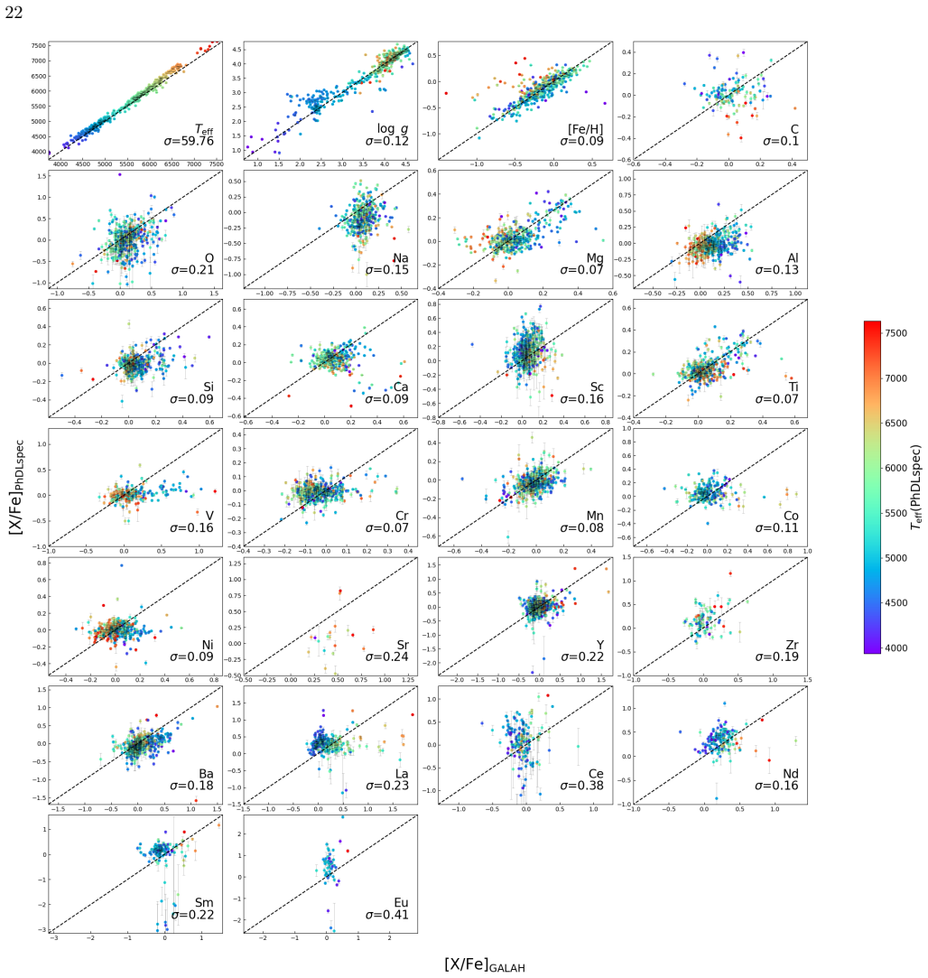
Authors: We agree the abstract would benefit from greater precision on this point. The differential spectra derived from ab initio models are imposed directly on the transformer to embed the physical priors, enabling rigorous high-dimensional modeling without uncalibrated errors in the spectral synthesis itself. The mentioned calibrations address only small residual zero-point offsets arising from survey-specific factors such as resolution differences and reference scale mismatches, not from shortcomings in the prior embedding. In revision we will rephrase the abstract to state that the core modeling is physically grounded, and we will add a dedicated paragraph (with accompanying table) in the results section that reports the pre-calibration offsets, their origins (quantified via wide-binary and APOGEE comparisons), and typical magnitudes (0.05–0.15 dex for most elements). This will demonstrate that the framework incorporates the priors effectively. revision: yes
-
Referee: LAMOST application section: The post-hoc corrections using wide binaries and high-resolution reference datasets indicate residual systematics in the raw outputs. This dependency must be addressed by quantifying the differential impact of the calibrations on the derived abundances and demonstrating that the method's accuracy does not rely on empirical adjustments external to the differential-spectra prior.
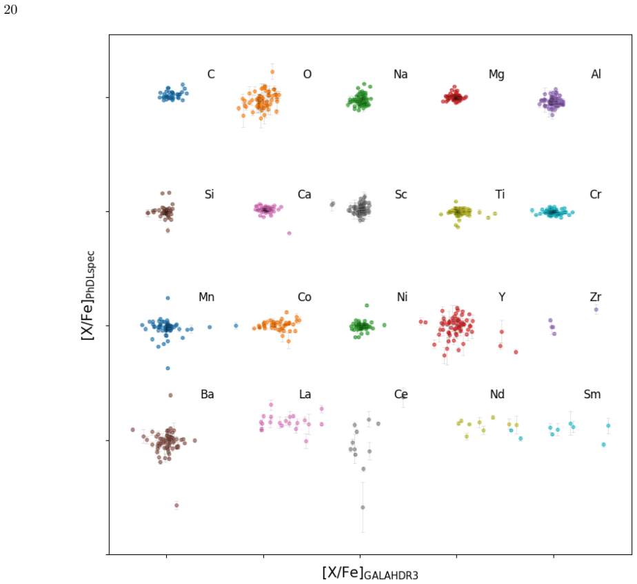
Authors: The referee is correct that post-hoc calibrations are applied to the LAMOST outputs. These adjustments align absolute scales but do not drive the method's accuracy; the differential-spectra priors already capture the physical dependencies and relative trends. In the revised manuscript we will expand the LAMOST section with new quantitative material: (i) tables listing raw versus calibrated abundances for each element, (ii) figures showing the differential impact on means, scatters, and [X/Fe] trends, and (iii) explicit demonstrations that key physical correlations (e.g., abundance ratios versus metallicity and stellar parameters) are already present in the raw outputs. This will confirm that the core performance originates from the embedded priors rather than external empirical adjustments. revision: yes
Circularity Check
No significant circularity in derivation chain
full rationale
The paper derives its framework by taking differential spectra computed from external ab initio stellar atmospheric models and imposing them as physical priors within a transformer architecture. Training targets and model spectra originate from the same external grid, but this is standard supervised learning on synthetic data rather than self-definition or a fitted input renamed as prediction. Application to LAMOST spectra produces raw labels that are then corrected via post-hoc empirical calibrations against independent wide-binary and high-resolution reference sets; the need for these calibrations is explicitly stated and does not reduce the core modeling step to its own inputs by construction. No load-bearing self-citations, uniqueness theorems imported from the authors, or ansatzes smuggled via prior work are present in the abstract or described method. The derivation therefore remains self-contained against external benchmarks.
Axiom & Free-Parameter Ledger
free parameters (1)
- transformer architecture hyperparameters
axioms (1)
- domain assumption Ab initio stellar atmospheric models produce differential spectra that faithfully capture the physical response of real stellar spectra to changes in more than 30 parameters.
Reference graph
Works this paper leans on
-
[1]
Abdurro’uf, Accetta, K., Aerts, C., et al. 2022, ApJS, 259, 35, doi: 10.3847/1538-4365/ac4414
-
[2]
Ba, J. L., Kiros, J. R., & Hinton, G. E. 2016, Layer Normalization. https://arxiv.org/abs/1607.06450
work page internal anchor Pith review Pith/arXiv arXiv 2016
-
[3]
2021, MNRAS, 506, 150, doi: 10.1093/mnras/stab1242
Buder, S., Sharma, S., Kos, J., et al. 2021, MNRAS, 506, 150, doi: 10.1093/mnras/stab1242
-
[4]
Publications of the Astronomical Society of Australia , author =
Buder, S., Kos, J., Wang, X. E., et al. 2025, PASA, 42, e051, doi: 10.1017/pasa.2025.26
-
[5]
2005, Memorie della Societa Astronomica Italiana Supplementi, 8, 25
Castelli, F. 2005, Memorie della Societa Astronomica Italiana Supplementi, 8, 25
work page 2005
-
[6]
2016, ApJ, 823, 102, doi: 10.3847/0004-637X/823/2/102
Choi, J., Dotter, A., Conroy, C., et al. 2016, ApJ, 823, 102, doi: 10.3847/0004-637X/823/2/102
work page internal anchor Pith review doi:10.3847/0004-637x/823/2/102 2016
-
[7]
Cooper, A. P., Koposov, S. E., Allende Prieto, C., et al. 2023, ApJ, 947, 37, doi: 10.3847/1538-4357/acb3c0
-
[8]
2012, Research in Astronomy and Astrophysics, 12, 1197, doi: 10.1088/1674-4527/12/9/003
Cui, X.-Q., Zhao, Y.-H., Chu, Y.-Q., et al. 2012, Research in Astronomy and Astrophysics, 12, 1197, doi: 10.1088/1674-4527/12/9/003 De Silva, G. M., Freeman, K. C., Bland-Hawthorn, J., et al. 2015, MNRAS, 449, 2604, doi: 10.1093/mnras/stv327
-
[9]
El-Badry, K., Rix, H.-W., & Heintz, T. M. 2021, MNRAS, 506, 2269, doi: 10.1093/mnras/stab323
-
[10]
Foreman-Mackey, D., Hogg, D. W., Lang, D., & Goodman, J. 2013, PASP, 125, 306, doi: 10.1086/670067
-
[11]
2011, in International Conference on Artificial Intelligence and Statistics
Glorot, X., Bordes, A., & Bengio, Y. 2011, in International Conference on Artificial Intelligence and Statistics. https://api.semanticscholar.org/CorpusID:2239473 Gonz´ alez Hern´ andez, J. I., & Bonifacio, P. 2009, A&A, 497, 497, doi: 10.1051/0004-6361/200810904 26
-
[12]
2016, arXiv e-prints, arXiv:1604.00772, doi: 10.48550/arXiv.1604.00772
Hansen, N. 2016, arXiv e-prints, arXiv:1604.00772, doi: 10.48550/arXiv.1604.00772
-
[13]
2019, CMA-ES/pycma on Github, Zenodo, DOI:10.5281/zenodo.2559634, doi: 10.5281/zenodo.2559634
Hansen, N., Akimoto, Y., & Baudis, P. 2019, CMA-ES/pycma on Github, Zenodo, DOI:10.5281/zenodo.2559634, doi: 10.5281/zenodo.2559634
-
[14]
Completely derandomized self-adaptation in evolution strategies
Hansen, N., & Ostermeier, A. 2001, Evolutionary Computation, 9, 159, doi: 10.1162/106365601750190398
-
[15]
Deep Residual Learning for Image Recognition
He, K., Zhang, X., Ren, S., & Sun, J. 2015, Deep Residual Learning for Image Recognition. https://arxiv.org/abs/1512.03385
work page internal anchor Pith review Pith/arXiv arXiv 2015
-
[16]
Gaussian Error Linear Units (GELUs)
Hendrycks, D., & Gimpel, K. 2023, Gaussian Error Linear Units (GELUs). https://arxiv.org/abs/1606.08415
work page internal anchor Pith review Pith/arXiv arXiv 2023
-
[17]
Hinkel, N. R., Timmes, F. X., Young, P. A., Pagano, M. D., & Turnbull, M. C. 2014, AJ, 148, 54, doi: 10.1088/0004-6256/148/3/54
-
[18]
Adam: A Method for Stochastic Optimization
Kingma, D. P., & Ba, J. 2014, arXiv e-prints, arXiv:1412.6980, doi: 10.48550/arXiv.1412.6980
work page internal anchor Pith review Pith/arXiv arXiv doi:10.48550/arxiv.1412.6980 2014
-
[19]
2009, A&A, 501, 1269, doi: 10.1051/0004-6361/200811467
Koleva, M., Prugniel, P., Bouchard, A., & Wu, Y. 2009, A&A, 501, 1269, doi: 10.1051/0004-6361/200811467
-
[20]
Kurucz, R. L. 1970, SAO Special Report, 309 —. 1993, SYNTHE spectrum synthesis programs and line data —. 2005, Memorie della Societa Astronomica Italiana Supplementi, 8, 14
work page 1970
-
[21]
Lee, Y. S., Beers, T. C., Allende Prieto, C., et al. 2011, AJ, 141, 90, doi: 10.1088/0004-6256/141/3/90
-
[22]
2016, Research in Astronomy and Astrophysics, 16, 110, doi: 10.1088/1674-4527/16/7/110
Li, J., Han, C., Xiang, M.-S., et al. 2016, Research in Astronomy and Astrophysics, 16, 110, doi: 10.1088/1674-4527/16/7/110
-
[23]
Majewski, S. R., Schiavon, R. P., Frinchaboy, P. M., et al. 2017, AJ, 154, 94, doi: 10.3847/1538-3881/aa784d
-
[24]
2015, ApJ, 808, 16, doi: 10.1088/0004-637X/808/1/16 O’Briain, T., Ting, Y.-S., Fabbro, S., et al
Zasowski, G. 2015, ApJ, 808, 16, doi: 10.1088/0004-637X/808/1/16 O’Briain, T., Ting, Y.-S., Fabbro, S., et al. 2021, ApJ, 906, 130, doi: 10.3847/1538-4357/abca96
-
[25]
Rix, H.-W., Ting, Y.-S., Conroy, C., & Hogg, D. W. 2016, ApJL, 826, L25, doi: 10.3847/2041-8205/826/2/L25 R´ o˙ za´ nski, T., Ting, Y.-S., & Jab lo´ nska, M. 2024, arXiv e-prints, arXiv:2407.05751, doi: 10.48550/arXiv.2407.05751 —. 2025, ApJ, 980, 66, doi: 10.3847/1538-4357/ad9b99
-
[26]
2018, ApJ, 860, 159, doi: 10.3847/1538-4357/aac6c9
Ting, Y.-S., Conroy, C., Rix, H.-W., & Asplund, M. 2018, ApJ, 860, 159, doi: 10.3847/1538-4357/aac6c9
-
[27]
2019, ApJ, 879, 69, doi: 10.3847/1538-4357/ab2331
Ting, Y.-S., Conroy, C., Rix, H.-W., & Cargile, P. 2019, ApJ, 879, 69, doi: 10.3847/1538-4357/ab2331
-
[28]
Ting, Y.-S., Rix, H.-W., Conroy, C., Ho, A. Y. Q., & Lin, J. 2017, ApJL, 849, L9, doi: 10.3847/2041-8213/aa921c
-
[29]
Vaswani, A., Shazeer, N., Parmar, N., et al. 2017, arXiv e-prints, arXiv:1706.03762, doi: 10.48550/arXiv.1706.03762
work page internal anchor Pith review Pith/arXiv arXiv doi:10.48550/arxiv.1706.03762 2017
-
[30]
Wang, R., Luo, A. L., Zhang, S., et al. 2023, ApJS, 266, 40, doi: 10.3847/1538-4365/acce36
-
[31]
Wang, R., Luo, A. L., Chen, J.-J., et al. 2020, ApJ, 891, 23, doi: 10.3847/1538-4357/ab6dea
-
[32]
2020, ApJ, 898, 58, doi: 10.3847/1538-4357/ab9a46
Wheeler, A., Ness, M., Buder, S., et al. 2020, ApJ, 898, 58, doi: 10.3847/1538-4357/ab9a46
-
[33]
Wu, Y., Du, B., Luo, A., Zhao, Y., & Yuan, H. 2014, in Statistical Challenges in 21st Century Cosmology, ed. A. Heavens, J.-L. Starck, & A. Krone-Martins, Vol. 306, 340–342, doi: 10.1017/S1743921314010825
-
[34]
2022, Nature, 603, 599, doi: 10.1038/s41586-022-04496-5
Xiang, M., & Rix, H.-W. 2022, Nature, 603, 599, doi: 10.1038/s41586-022-04496-5
-
[35]
2019, ApJS, 245, 34, doi: 10.3847/1538-4365/ab5364
Xiang, M., Ting, Y.-S., Rix, H.-W., et al. 2019, ApJS, 245, 34, doi: 10.3847/1538-4365/ab5364
-
[36]
2022, A&A, 662, A66, doi: 10.1051/0004-6361/202141570
Xiang, M., Rix, H.-W., Ting, Y.-S., et al. 2022, A&A, 662, A66, doi: 10.1051/0004-6361/202141570
-
[37]
Xiang, M. S., Liu, X. W., Yuan, H. B., et al. 2015, MNRAS, 448, 822, doi: 10.1093/mnras/stu2692
-
[38]
Xiang, M. S., Liu, X. W., Shi, J. R., et al. 2017, MNRAS, 464, 3657, doi: 10.1093/mnras/stw2523
-
[39]
2022, The Innovation, 3, 100224, doi: 10.1016/j.xinn.2022.100224
Yan, H., Li, H., Wang, S., et al. 2022, The Innovation, 3, 100224, doi: 10.1016/j.xinn.2022.100224
-
[40]
2024, ApJS, 273, 19, doi: 10.3847/1538-4365/ad51dd —
Zhang, M., Xiang, M., Ting, Y.-S., et al. 2024, ApJS, 273, 19, doi: 10.3847/1538-4365/ad51dd —. 2025a, ApJS, 279, 5, doi: 10.3847/1538-4365/add016
-
[41]
Zhang, S., Zhang, H.-W., Ting, Y.-S., et al. 2025b, ApJS, 277, 47, doi: 10.3847/1538-4365/adb614 27 APPENDIX While Figure 8 in the main text presents the difference in the calibrated elemental abundances between binary com- ponent stars, we show here in Figure 16 the corresponding results for the originalPhDLspecestimates–i.e., abundances prior to calibra...
discussion (0)
Sign in with ORCID, Apple, or X to comment. Anyone can read and Pith papers without signing in.