Legendrian position of veering triangulations
Pith reviewed 2026-05-10 17:16 UTC · model grok-4.3
The pith
Veering triangulations can be positioned so their edges are Legendrian arcs in a bicontact structure supporting the Anosov flow.
A machine-rendered reading of the paper's core claim, the machinery that carries it, and where it could break.
Core claim
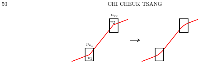
Given a veering triangulation corresponding to an Anosov flow with orientable stable and unstable foliations, the edges of the triangulation can be realized as Legendrian arcs with respect to a strongly adapted bicontact structure that supports the Anosov flow. Every veering triangulation can be placed in steady position, where each pair of edge projections that intersect in the orbit space only intersect once transversely.
What carries the argument
The steady position, in which intersecting edge projections cross transversely only once, which facilitates the Legendrian realization.
If this is right
- Horizontal surgery of veering triangulations corresponds to horizontal Goodman surgery of pseudo-Anosov flows.
- This equivalence allows combinatorial changes to the triangulation to be translated directly into modifications of the flow.
- The Legendrian property is preserved under these operations.
Where Pith is reading between the lines
- This positioning might enable the use of Legendrian knot theory techniques to study properties of the Anosov flows.
- Steady position could simplify the analysis of intersection patterns in the orbit space for related combinatorial objects.
- The result may inspire similar Legendrian realizations for other types of triangulations or flows.
Load-bearing premise
The veering triangulation must correspond to an Anosov flow whose stable and unstable foliations are orientable, with a strongly adapted bicontact structure available to support it.
What would settle it
A concrete veering triangulation linked to such an Anosov flow in which no placement of the edges as Legendrian arcs exists under any strongly adapted bicontact structure, or where steady position cannot be achieved.
Figures


read the original abstract
We make a first step towards connecting the theory of veering triangulations and bicontact structures as tools for studying (pseudo-)Anosov flows: We show that given a veering triangulation corresponding to an Anosov flow with orientable stable and unstable foliations, the edges of the triangulation can be realized as Legendrian arcs with respect to a strongly adapted bicontact structure that supports the Anosov flow. Along the way, we show that every veering triangulation can be placed in `steady position', where each pair of edge projections that intersect in the orbit space only intersect once transversely. By a previous result of the author, this implies that horizontal surgery of veering triangulations correspond to horizontal Goodman surgery of pseudo-Anosov flows.
Editorial analysis
A structured set of objections, weighed in public.
Referee Report
Summary. The manuscript proves two main results connecting veering triangulations to bicontact structures and Anosov flows. Given a veering triangulation corresponding to an Anosov flow with orientable stable and unstable foliations, the edges can be realized as Legendrian arcs with respect to a strongly adapted bicontact structure supporting the flow. Separately, every veering triangulation admits a steady position in which any two edge projections that intersect in the orbit space do so exactly once and transversely. By a prior result of the author, the steady-position statement implies that horizontal surgery on veering triangulations corresponds to horizontal Goodman surgery on the associated pseudo-Anosov flows.
Significance. If the results hold, the work supplies a concrete geometric bridge between the combinatorial theory of veering triangulations and the contact-geometric theory of bicontact structures for Anosov flows. The unconditional steady-position theorem is likely to be useful on its own for controlling intersections in the orbit space. The Legendrian-realization statement is carefully scoped to the orientable-foliation case and to the existence of a strongly adapted bicontact structure, which keeps the claims falsifiable and proportionate to the tools employed.
minor comments (2)
- [Introduction] The introduction would benefit from a brief diagram or explicit coordinate description of the orbit space and the projection of edges, to make the definition of steady position immediately accessible to readers outside the immediate subfield.
- [Section 1] A short paragraph recalling the precise statement of the cited previous result on Goodman surgery would improve readability, even though the dependence is clearly flagged.
Simulated Author's Rebuttal
We thank the referee for their positive assessment of the manuscript, the clear summary of our results, and the recommendation to accept. We have no major comments to address.
Circularity Check
Minor self-citation for surgery implication; central Legendrian and steady-position results are independent
full rationale
The paper directly constructs the Legendrian realization of triangulation edges with respect to a strongly adapted bicontact structure (for the scoped case of Anosov flows with orientable foliations) and the steady position for arbitrary veering triangulations. These are presented as new results without reduction to prior self-citations. The sole self-reference is the sentence 'By a previous result of the author, this implies that horizontal surgery of veering triangulations correspond to horizontal Goodman surgery of pseudo-Anosov flows,' which applies only to an additional implication and is not used to justify the main theorems. No self-definitional loops, fitted inputs renamed as predictions, ansatz smuggling, or uniqueness theorems imported from the author's prior work appear in the derivation of the primary claims. The assumptions are explicitly stated and external to the self-citation.
Axiom & Free-Parameter Ledger
Reference graph
Works this paper leans on
-
[1]
[AT25a] Antonio Alfieri and Chi Cheuk Tsang
doi:10.2140/agt.2024.24.3401. [AT25a] Antonio Alfieri and Chi Cheuk Tsang. Heegaard floer theory and pseudo-anosov flows i: Generators and categorification of the zeta function,
-
[2]
[AT25b] Antonio Alfieri and Chi Cheuk Tsang
URL: https://arxiv.org/ abs/2504.15420,arXiv:2504.15420. [AT25b] Antonio Alfieri and Chi Cheuk Tsang. Heegaard floer theory and pseudo-anosov flows ii: Differential and fried pants,
-
[3]
[BBM24] Thomas Barthelm´ e, Christian Bonatti, and Kathryn Mann
URL: https://arxiv.org/abs/2506.07163, arXiv: 2506.07163. [BBM24] Thomas Barthelm´ e, Christian Bonatti, and Kathryn Mann. Non-transitive pseudo-Anosov flows,
-
[4]
Non-transitive pseudo- A nosov flows
URL:https://arxiv.org/abs/2411.03586,arXiv:2411.03586. [BFM25] Thomas Barthelm´ e, Steven Frankel, and Kathryn Mann. Orbit equivalences of pseudo- Anosov flows.Invent. Math., 240(3):1119–1192,
-
[5]
[BM26] Thomas Barthelm´ e and Kathryn Mann
doi:10.1007/s00222-025-01332-1 . [BM26] Thomas Barthelm´ e and Kathryn Mann. Pseudo-anosov flows: A plane approach,
-
[6]
URL:https://arxiv.org/abs/2509.15375,arXiv:2509.15375. [Bru95] Marco Brunella. Surfaces of section for expansive flows on three-manifolds.J. Math. Soc. Japan, 47(3):491–501, 1995.doi:10.2969/jmsj/04730491. [Cal00] Danny Calegari. The geometry ofR-covered foliations.Geom. Topol., 4:457–515,
-
[7]
[CLMM22] Kai Cieliebak, Oleg Lazarev, Thomas Massoni, and Agustin Moreno
doi:10.2140/gt.2000.4.457. [CLMM22] Kai Cieliebak, Oleg Lazarev, Thomas Massoni, and Agustin Moreno. Floer theory of anosov flows in dimension three,
- [8]
-
[9]
doi: 10.1007/s00014-002-8348-9. [Fen16] S´ ergio R. Fenley. Quasigeodesic pseudo-Anosov flows in hyperbolic 3-manifolds and con- nections with large scale geometry.Adv. Math., 303:192–278,
-
[10]
doi:10.1016/j.aim. 2016.05.015. [FH19] Todd Fisher and Boris Hasselblatt.Hyperbolic flows. Zurich Lectures in Advanced Mathe- matics. EMS Publishing House, Berlin, [2019]©2019.doi:10.4171/200. [FL25] Steven Frankel and Michael Landry. From quasigeodesic to pseudo-anosov flows,
-
[11]
URL:https://arxiv.org/abs/2510.02217,arXiv:2510.02217. [FLP12] Albert Fathi, Fran¸ cois Laudenbach, and Valentin Po´ enaru.Thurston’s work on surfaces, vol- ume 48 ofMathematical Notes. Princeton University Press, Princeton, NJ,
-
[12]
Translated from the 1979 French original by Djun M. Kim and Dan Margalit. [FSS25] Steven Frankel, Saul Schleimer, and Henry Segerman. From veering triangulations to link spaces and back again,
work page 1979
-
[13]
URL: https://arxiv.org/abs/1911.00006, arXiv: 1911.00006. [Hal25] Layne Hall. Recognising perfect fits,
-
[14]
URL: https://arxiv.org/abs/2501.00232, arXiv:2501.00232. [Hoz24] Surena Hozoori. Symplectic geometry of Anosov flows in dimension 3 and bi-contact topology.Adv. Math., 450:Paper No. 109764, 41,
-
[15]
doi:10.1016/j.aim.2024.109764. [Hoz25] Surena Hozoori. Strongly adapted contact geometry of Anosov 3-flows.J. Fixed Point Theory Appl., 27(2):Paper No. 37, 37, 2025.doi:10.1007/s11784-025-01180-9. [Iak22] Ioannis Iakovoglou. A new combinatorial invariant caracterizing anosov flows on 3-manifolds,
-
[16]
URL:https://arxiv.org/abs/2212.13177,arXiv:2212.13177. [Iak25] Ioannis Iakovoglou. Markovian families for pseudo-anosov flows,
-
[17]
60 CHI CHEUK TSANG [LMT23] Michael P
URL: https:// arxiv.org/abs/2509.19530,arXiv:2509.19530. 60 CHI CHEUK TSANG [LMT23] Michael P. Landry, Yair N. Minsky, and Samuel J. Taylor. Flows, growth rates, and the veering polynomial.Ergodic Theory Dynam. Systems, 43(9):3026–3107,
-
[18]
doi: 10.1017/etds.2022.63. [Mas25] Thomas Massoni. Anosov flows and Liouville pairs in dimension three.Algebr. Geom. Topol., 25(3):1793–1838, 2025.doi:10.2140/agt.2025.25.1793. [Mit95] Yoshihiko Mitsumatsu. Anosov flows and non-Stein symplectic manifolds.Ann. Inst. Fourier (Grenoble), 45(5):1407–1421,
-
[19]
Surgery on Anosov flows using bi-contact geometry.Ergodic Theory Dynam
[Sal25] Federico Salmoiraghi. Surgery on Anosov flows using bi-contact geometry.Ergodic Theory Dynam. Systems, 45(12):3832–3864, 2025.doi:10.1017/etds.2025.10196. [Sha21] Mario Shannon. Hyperbolic models for transitive topological anosov flows in dimension three, 2021.arXiv:2108.12000. [SS23] Saul Schleimer and Henry Segerman. From veering triangulations ...
-
[20]
[SS24] Saul Schleimer and Henry Segerman
arXiv:2305.08799. [SS24] Saul Schleimer and Henry Segerman. From loom spaces to veering triangulations.Groups Geom. Dyn., 18(2):419–462, 2024.doi:10.4171/ggd/742. [Tsa23a] Chi Cheuk Tsang. Veering branched surfaces, surgeries, and geodesic flows.New York J. Math., 29:1425–1495,
-
[21]
URL: https://www.proquest.com/dissertations-theses/ veering-triangulations-pseudo-anosov-flows/docview/2869041415/se-2. [Tsa24a] Chi Cheuk Tsang. Constructing Birkhoff sections for pseudo-Anosov flows with controlled complexity.Ergodic Theory Dynam. Systems, 44(8):2308–2360,
-
[22]
doi:10.1017/etds. 2023.105. [Tsa24b] Chi Cheuk Tsang. Examples of anosov flows with genus one birkhoff sections,
-
[23]
URL: https://arxiv.org/abs/2402.00229,arXiv:2402.00229. [Tsa24c] Chi Cheuk Tsang. Horizontal goodman surgery and almost equivalence of pseudo-anosov flows, 2024.arXiv:2401.01847. [Zun] Jonathan Zung. Anosov flows and the pair of pants differential. In preparation. Email address:chicheuk@hotmail.com
discussion (0)
Sign in with ORCID, Apple, or X to comment. Anyone can read and Pith papers without signing in.