Restricted Search Space Graph MCMC via Birth-Death Processes
Pith reviewed 2026-05-10 16:41 UTC · model grok-4.3
The pith
Sharp bounds quantify the total variation error from restricting the edge search space in MCMC for inferring directed acyclic graphs, while a birth-death process allows the restriction to grow or shrink dynamically.
A machine-rendered reading of the paper's core claim, the machinery that carries it, and where it could break.
Core claim
We derive sharp lower and upper bounds on the total variation distance between the unrestricted posterior distribution and the posterior distribution induced by a state-of-the-art restricted search space MCMC method. These bounds characterize regimes in which the approximation error is negligible and regimes in which it is not. In order to reduce the error, we propose a flexible transdimensional MCMC sampler which allows the search space to expand or contract dynamically as the chain progresses. The sampler is defined by birth-and-death rates that induce a prior distribution on the set of search spaces, rather than assume a fixed restricted search space throughout.
What carries the argument
Birth-and-death rates that induce a prior over possible restricted search spaces, thereby driving a transdimensional MCMC chain whose edge set can change during sampling.
Load-bearing premise
That birth-and-death rates can be chosen to induce a prior on search spaces such that the resulting transdimensional chain mixes well and the approximation error remains controlled without introducing new intractable computations.
What would settle it
For a small DAG whose exact posterior can be enumerated, run both the fixed-restriction and the dynamic birth-death samplers and check whether the empirical total variation distance to the true posterior exceeds the derived upper bound.
Figures


read the original abstract
Inferring directed acyclic graphs (DAGs) from data via Markov chain Monte Carlo (MCMC) is computationally challenging in moderate-to-high dimensional settings because their discrete sampling space grows super-exponentially with the number of nodes. To address scalability, several recent MCMC-based graph inference methods restrict the search space to a subset of edges, at the cost of introducing error into the inference procedure. In this work, we derive sharp lower and upper bounds on the total variation distance between the unrestricted posterior distribution and the posterior distribution induced by a state-of-the-art restricted search space MCMC method. These bounds characterize regimes in which the approximation error is negligible and regimes in which it is not. In order to reduce the error, we propose a flexible transdimensional MCMC sampler which allows the search space to expand or contract dynamically as the chain progresses. The sampler is defined by birth-and-death rates that induce a prior distribution on the set of search spaces, rather than assume a fixed restricted search space throughout. We outline an efficient implementation of the proposed algorithm and demonstrate its finite-sample performance through simulation studies.
Editorial analysis
A structured set of objections, weighed in public.
Referee Report
Summary. The paper derives sharp lower and upper bounds on the total variation distance between the unrestricted posterior over DAGs and the posterior induced by a fixed restricted-search-space MCMC sampler. It then proposes a transdimensional birth-death MCMC sampler whose birth and death rates induce a prior over possible search spaces, allowing the restriction to expand or contract dynamically, and outlines an efficient implementation whose finite-sample behavior is illustrated via simulation studies.
Significance. If the TV bounds are indeed sharp and the birth-death construction preserves the exact marginal posterior on graphs while remaining computationally tractable, the work would provide a principled way to control approximation error in scalable Bayesian DAG inference. The explicit bounds and the dynamic-search-space idea are potentially valuable contributions to the literature on structure learning.
major comments (3)
- [Section describing the birth-death construction and implementation outline] The TV bounds are stated for a fixed restricted search space. For the dynamic sampler, the marginal posterior on graphs remains exactly the target only if the birth-death rates are chosen so that detailed balance holds for the joint (graph, search-space) process. The manuscript must exhibit the explicit functional form of these rates and prove that they can be evaluated without computing the normalizing constant over admissible search spaces or the posterior mass outside any candidate space (see the skeptic note on rate selection).
- [Implementation outline and simulation studies] The abstract claims an 'efficient implementation' exists and that the approximation error can be controlled. However, the provided outline does not include an error analysis showing that the induced prior keeps the TV distance within the derived bounds for the dynamic case, nor does it demonstrate that the rates remain posterior-independent. This is load-bearing for the central claim that the method reduces error without reintroducing intractability.
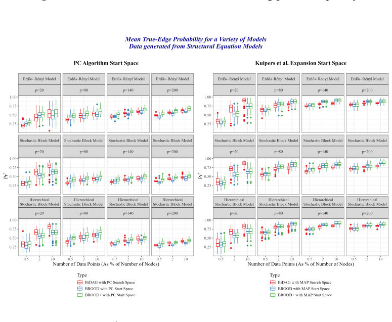
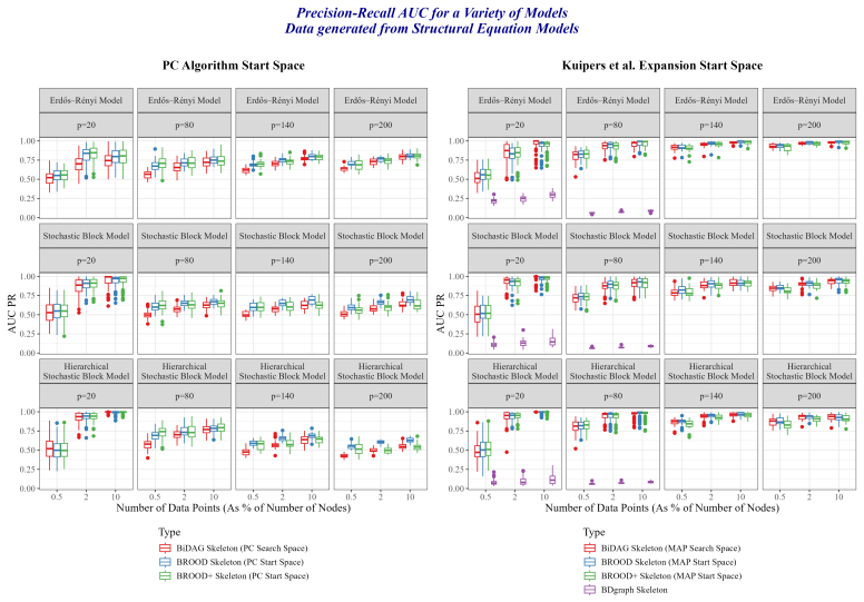
- [Simulation studies] Simulation studies are used to demonstrate finite-sample performance, but without reporting the realized TV distance (or a proxy) against the theoretical bounds, or comparing against a fixed-restriction baseline under the same computational budget, it is difficult to assess whether the dynamic adjustment actually improves upon the static case in the regimes the bounds identify as problematic.
minor comments (1)
- Notation for the collection of admissible search spaces and the induced prior should be introduced earlier and used consistently when stating the TV bounds.
Simulated Author's Rebuttal
We are grateful to the referee for their insightful comments and recommendations. Below we provide point-by-point responses to the major comments and outline the revisions we will undertake.
read point-by-point responses
-
Referee: [Section describing the birth-death construction and implementation outline] The TV bounds are stated for a fixed restricted search space. For the dynamic sampler, the marginal posterior on graphs remains exactly the target only if the birth-death rates are chosen so that detailed balance holds for the joint (graph, search-space) process. The manuscript must exhibit the explicit functional form of these rates and prove that they can be evaluated without computing the normalizing constant over admissible search spaces or the posterior mass outside any candidate space (see the skeptic note on rate selection).
Authors: We agree that the explicit rates and detailed balance for the joint process are necessary to establish the exact marginal posterior. In the revised manuscript we will state the functional forms of the birth and death rates explicitly and supply the proof that these rates satisfy detailed balance while depending only on the current graph, the current search space, and the induced prior; no global normalizing constant or mass outside the candidate space is required. revision: yes
-
Referee: [Implementation outline and simulation studies] The abstract claims an 'efficient implementation' exists and that the approximation error can be controlled. However, the provided outline does not include an error analysis showing that the induced prior keeps the TV distance within the derived bounds for the dynamic case, nor does it demonstrate that the rates remain posterior-independent. This is load-bearing for the central claim that the method reduces error without reintroducing intractability.
Authors: We acknowledge that the outline in the current draft is concise. The revision will expand the implementation section with an explicit error analysis showing that the dynamic prior keeps the total-variation distance inside the derived bounds, and will demonstrate that the rates are posterior-independent by construction, depending solely on the current state and the prior over search spaces. revision: yes
-
Referee: [Simulation studies] Simulation studies are used to demonstrate finite-sample performance, but without reporting the realized TV distance (or a proxy) against the theoretical bounds, or comparing against a fixed-restriction baseline under the same computational budget, it is difficult to assess whether the dynamic adjustment actually improves upon the static case in the regimes the bounds identify as problematic.
Authors: We agree that direct numerical checks against the bounds and matched-budget comparisons would strengthen the empirical section. The revised simulation studies will report realized TV distances (or computable proxies) and will add comparisons to fixed-restriction samplers under identical computational budgets, focusing on the regimes identified by the bounds. revision: yes
Circularity Check
No circularity: TV bounds and birth-death sampler derived independently of fitted inputs or self-citation chains
full rationale
The paper's core contributions are a mathematical derivation of sharp TV distance bounds between unrestricted and restricted posteriors, plus a direct construction of a transdimensional sampler via birth-death rates that induce a prior on search spaces. No equations or steps reduce the claimed bounds or sampler performance to quantities defined from the same data by construction, nor do they rely on load-bearing self-citations whose validity is assumed without external verification. The abstract and described claims treat the bounds as new characterizations and the rates as a flexible proposal with an outlined efficient implementation, keeping the derivation self-contained against external benchmarks.
Axiom & Free-Parameter Ledger
axioms (1)
- domain assumption Birth-and-death rates induce a prior distribution on the set of search spaces
Reference graph
Works this paper leans on
-
[1]
Morgan Kaufmann, San Francisco (CA). Byrne, S. and Dawid, A. P. (2015). Structural Markov graph laws for Bayesian model uncertainty.The Annals of Statistics, 43(4):1647–1681. Cao,X.,Khare,K.,andGhosh,M.(2019). Posteriorgraphselectionandestimationconsis- tency for high-dimensional Bayesian DAG models.The Annals of Statistics, 47(1):319– 348. Caron, A., Lia...
-
[2]
banned” score table tabulating all of the valid scores that arecompatiblewithparticular“banned
We will do so now, showing thatγis well-defined for any 2 random edges outside of EH,e 1, e2. We need to show that b(θ(H+e1 ,≺), θe2) D(θ(H+e1 ,≺), θe2) b(θ(H,≺), θe1) D(θ(H,≺), θe1) = b(θ(H+e2 ,≺), θe1) D(θ(H+e2 ,≺), θe1) b(θ(H,≺), θe2) D(θ(H,≺), θe2) (32) To prove 32, we define the following 4 disjoint sets of graphs: G0 :={G:G∈ G H} G1 :={G:e 1 ∈G, G∈ ...
work page 1977
-
[3]
banned” score table takesO(2Kp)to compute. Creating the plus “banned
score tables takeO(K3p2K)to compute, BGe plus score tables takeO(K3p2K(p− K−1))tocompute(byrepeatingthescoretableprocessforeachofthe(p− |pa H(i)| −1) excluded nodes fromH, and the “banned” score table takesO(2Kp)to compute. Creating the plus “banned” score table is alsoO(2Kp), as the row-matching process to create theBi values illustrated in table 1 can b...
work page 2014
-
[4]
A single-block cluster withmin(0.1,4 p)connection probability
-
[5]
A two-block cluster with(1 3 , 2 3)probability of assignment and the same connection probability matrix as the SBM in (38)
-
[6]
This hierarchical design yields graphs with both community and anti-community structure
Athree-blockclusterwith( 1 6 , 1 3 , 1 2)probabilityofassignmentandaconnectionprob- ability matrix of min(0.2, 8 p) min(0.01, 1 p) min(0.2, 8 p) min(0.01, 1 p) 0 min(0.08, 4 p) min(0.2, 8 p) min(0.08, 4 p) min(0.08, 4 p) The third cluster introduces more complex relationships both within and between blocks; while blocks 1 and 3 within this setup e...
work page 2021
discussion (0)
Sign in with ORCID, Apple, or X to comment. Anyone can read and Pith papers without signing in.