Layered Control of Partially Observed Stochastic Systems

Anastasios Tsiamis; Charis Stamouli; George J. Pappas

arxiv: 2604.11956 · v1 · submitted 2026-04-13 · 📡 eess.SY · cs.SY

Layered Control of Partially Observed Stochastic Systems

Charis Stamouli , Anastasios Tsiamis , George J. Pappas This is my paper

Pith reviewed 2026-05-10 15:12 UTC · model grok-4.3

classification 📡 eess.SY cs.SY

keywords layered controlpartial observationsstochastic systemssimulation functionsKalman estimatorhierarchical controlaerial robotics

0 comments

The pith

Stochastic simulation functions bound expected output distances between layers in partially observed stochastic systems.

A machine-rendered reading of the paper's core claim, the machinery that carries it, and where it could break.

The paper develops a layered control method for stochastic systems that are only partially observed. It defines stochastic simulation functions that incorporate state estimators at each layer to ensure the expected output distance between a detailed lower-layer system and a coarser upper-layer system stays below a bound that can be calculated in advance. A reader would care because this supplies performance guarantees when breaking complex noisy systems into simpler hierarchical layers. The construction is made explicit for linear systems that use Kalman filters at every level, and the framework is shown on two aerial robot examples.

Core claim

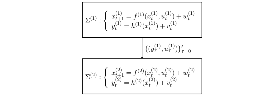
The central claim is that stochastic simulation functions can be defined for partially observed stochastic systems such that, whenever one system simulates the other via the supplied estimators, the expected distance between their outputs remains bounded by a quantity computable from the initial states and the estimator parameters. For linear systems the functions are constructed directly from the system matrices and the Kalman filter gains, and these functions are then used to synthesize controllers that respect the layer bounds.

What carries the argument

Stochastic simulation function for partially observed systems, which certifies that the expected output deviation between two systems is bounded once state estimators are given at each layer.

If this is right

Explicit constructions exist for linear systems using system matrices and Kalman gains.
Controllers can be synthesized that keep layer-wise output errors inside the certified bounds.
The bounds are computable ahead of time, permitting verification of layer compatibility before deployment.
The method is demonstrated on an unmanned aerial vehicle and a hexacopter carrying a camera.

Where Pith is reading between the lines

These are editorial extensions of the paper, not claims the author makes directly.

The same bounding technique could be tried with nonlinear estimators once they are supplied at each layer.
It points toward abstraction-based planning for robotic systems where uncertainty grows with model coarseness.
One could measure how loose the bounds become when the layers differ greatly in dimension or dynamics.

Load-bearing premise

Suitable state estimators such as Kalman filters are already provided at each layer.

What would settle it

A linear system together with its Kalman estimator for which the actual expected output distance between layers exceeds the bound given by the constructed stochastic simulation function.

Figures

Figures reproduced from arXiv: 2604.11956 by Anastasios Tsiamis, Charis Stamouli, George J. Pappas.

**Figure 1.** Figure 1: Two-layer control architecture for partially observed stochastic systems. Our goal is to control system Σ(2) so that it approximates the output behavior of Σ(1) under any controller within guaranteed computable bounds. • We propose a principled framework for layered control of partially observed stochastic systems. • Our framework relies on novel stochastic simulation functions tailored to partially observ… view at source ↗

**Figure 2.** Figure 2: Two-layer control architecture with partially observed stochastic linear systems. The Kalman state estimate ˆx (1) t depends on the observed sequence {(y (1) τ , u (1) t )} t−1 τ=0 [PITH_FULL_IMAGE:figures/full_fig_p005_2.png] view at source ↗

**Figure 3.** Figure 3: Illustration of the two aerial robot architectures. 5.1 Unmanned Aerial Vehicle (UAV) Consider a small fixed-wing UAV whose longitudinal dynamics are modeled with a linearized system Σ (1) from [21]. The state is x (1) := (V (1), a(1), ω (1) θ , θ(1)), where V (1) ∈ R is the airspeed, a (1) ∈ R the angle of attack, θ (1) ∈ R the pitch angle, and ω (1) θ ∈ R the pitch angular rate. The input [PITH_FULL_IMA… view at source ↗

**Figure 4.** Figure 4: UAV with extra control surfaces. Left: Output distance of Σ(1) and Σ(2) for 20 individual trials, and average across 200 trials. We observe that ε is a quite tight bound for the average output distance over time. Right: Output norm of systems Σ(1) and Σ(2) for a single trial. As Σ(1) is stabilized, our layered control framework leads Σ(2) to stabilize as well. u (1) := (δθ, δt) consists of the pitch actuat… view at source ↗

**Figure 5.** Figure 5: Hexacopter with camera payload. Left: Output distance of Σ(1) and Σ(2) for 20 individual trials, and average across 200 trials. We observe that ε is a quite tight bound for the average output distance over time. Right: Output norm of systems Σ(1) and Σ(2) for a single trial. As Σ(1) is stabilized, our layered control framework leads Σ(2) to stabilize as well. and the altitude velocity v (1) z . The dynamic… view at source ↗

read the original abstract

Layered control is essential for managing complexity in large-scale systems, employing progressively coarser models at higher layers. While significant advances have been made for fully observable systems, the theoretical foundations of layered control under partial observations and stochastic noise remain underexplored. To address this gap, we propose a principled layered control framework for such settings. Given a state estimator at each layer, our approach ensures that the expected output distance between systems at successive layers remains within a priori computable bounds. This is achieved by introducing a novel notion of stochastic simulation functions for partially observed systems. For the class of linear systems with Kalman estimators, we provide a systematic construction of these functions along with the corresponding control design. We demonstrate our framework on two aerial robotic scenarios: an unmanned aerial vehicle and a hexacopter with a camera payload.

Editorial analysis

A structured set of objections, weighed in public.

Desk editor's note, referee report, simulated authors' rebuttal, and a circularity audit. Tearing a paper down is the easy half of reading it; the pith above is the substance, this is the friction.

Desk Editor's Note private letter to a colleague

The paper defines stochastic simulation functions for partially observed stochastic systems and gives an explicit construction for linear dynamics with Kalman estimators, which extends prior layered control work without obvious contradictions.

read the letter

This paper takes the existing layered control framework for fully observable systems and adapts it to the partial-observation stochastic case. The central move is a new definition of stochastic simulation functions that incorporate a state estimator at each layer, so that the expected output distance between successive layers stays inside a bound you can compute in advance. For linear systems they supply a concrete procedure using Kalman filters, and they close with two aerial-robot examples: a UAV and a hexacopter carrying a camera. That is the actual advance; the rest is standard control-theory scaffolding around it. The construction is stated clearly and the assumption that suitable estimators are already available is flagged up front, which keeps the claim honest. The examples are relevant to the robotics audience the authors target. The main limitation is the restriction to linear dynamics; nothing in the paper suggests an immediate route to nonlinear plants, so anyone wanting broader applicability will still need extra work. The robotic demonstrations are illustrative rather than exhaustive, with no large-scale Monte-Carlo quantification or direct comparison against non-layered baselines, but that is a matter of emphasis rather than a flaw in the argument. The paper is aimed at control theorists and roboticists who already think in terms of hierarchical or multi-layer architectures under uncertainty. A reader who needs a concrete way to certify bounds when observations are noisy will get usable definitions and a linear-case recipe. It is coherent on its own terms and addresses a gap that the abstract correctly identifies, so it merits a serious referee even if the nonlinear extension and tighter empirical validation are left for follow-up.

Referee Report

2 major / 2 minor

Summary. The paper proposes a layered control framework for partially observed stochastic systems. Given state estimators at each layer, it introduces a novel notion of stochastic simulation functions to ensure that the expected output distance between systems at successive layers remains within a priori computable bounds. For linear systems with Kalman estimators, the paper provides an explicit construction of these functions and the associated control design. The framework is demonstrated on two aerial robotic examples: an unmanned aerial vehicle and a hexacopter with a camera payload.

Significance. If the constructions and bounds hold, this work fills a notable gap by extending layered control theory to stochastic, partially observed settings that are prevalent in applications such as robotics. The explicit, systematic procedure for the linear case with Kalman filters, together with the use of simulation functions to derive computable bounds, offers a concrete tool for hierarchical design. The two robotic case studies provide initial evidence of applicability.

major comments (2)

[§3] §3 (Definition of stochastic simulation functions): The novel definition for partially observed systems is introduced to bound expected output distances, but the manuscript does not explicitly verify that the stochastic simulation relation is preserved under the Kalman estimator dynamics for the linear case; this step is load-bearing for the claim that bounds remain a priori computable across layers.
[§4] §4 (Construction for linear systems): The systematic construction of the simulation functions and control laws is presented for systems with given Kalman estimators, yet the derivation of the bound constants appears to rely on the estimator error covariance without showing that the constants remain finite and independent of the specific control policy chosen at each layer.

minor comments (2)

[Abstract] The abstract states that bounds are 'a priori computable,' but the main text should clarify whether these bounds depend on the choice of layer-specific controllers or remain uniform.
[Simulation section] Figure captions for the UAV and hexacopter examples should include the numerical values of the computed bounds to allow direct comparison with the simulation results.

Simulated Author's Rebuttal

2 responses · 0 unresolved

We thank the referee for the positive evaluation of the paper's significance and for the constructive major comments. We address each point below, agreeing that additional explicit verification and clarification will strengthen the manuscript. We will incorporate the suggested revisions in the next version.

read point-by-point responses

Referee: [§3] §3 (Definition of stochastic simulation functions): The novel definition for partially observed systems is introduced to bound expected output distances, but the manuscript does not explicitly verify that the stochastic simulation relation is preserved under the Kalman estimator dynamics for the linear case; this step is load-bearing for the claim that bounds remain a priori computable across layers.

Authors: We agree that an explicit verification of preservation under the Kalman estimator dynamics is necessary to fully support the a priori computability claim. In the revised manuscript, we will add a new lemma (Lemma 3.2) immediately following Definition 3.1 in Section 3. The lemma will prove that if a stochastic simulation function exists for the underlying linear system, then the relation is preserved when the lower-layer system is replaced by its Kalman estimator, with the output-distance bound expressed in terms of the estimator's error covariance. The proof will use the linearity of the dynamics, the orthogonality of the innovation process, and the fact that the estimation error is independent of the applied control input. This addition will make the load-bearing step fully explicit without altering the original definition. revision: yes
Referee: [§4] §4 (Construction for linear systems): The systematic construction of the simulation functions and control laws is presented for systems with given Kalman estimators, yet the derivation of the bound constants appears to rely on the estimator error covariance without showing that the constants remain finite and independent of the specific control policy chosen at each layer.

Authors: The estimator error covariance matrix P is obtained by solving the discrete algebraic Riccati equation offline using only the system matrices A, C and the noise covariances Q, R; it is therefore independent of any control policy applied at the current or higher layers. We will revise the opening paragraph of Section 4 and the statement of Theorem 4.1 to explicitly note this independence, provide the closed-form expression for the simulation-function constants in terms of the fixed P, and add a short remark explaining why the constants remain finite for any stabilizing Kalman gain. These changes will directly address the concern while preserving the existing constructions. revision: yes

Circularity Check

0 steps flagged

No significant circularity detected in derivation chain

full rationale

The paper defines a new notion of stochastic simulation functions for partially observed systems and, given state estimators (explicitly assumed, e.g., Kalman filters for linear cases), constructs them to bound expected output distances between layers. This is a definitional and constructive framework rather than a reduction of outputs to inputs by construction. No self-citation load-bearing steps, fitted parameters renamed as predictions, or ansatz smuggling via prior work are present in the provided text. The central claim rests on the stated assumptions and the novel definition, which is independent of the target bounds. The derivation is self-contained against external benchmarks.

Axiom & Free-Parameter Ledger

0 free parameters · 2 axioms · 1 invented entities

The framework rests on the new definition of stochastic simulation functions and the assumption that state estimators are supplied at each layer; no free parameters are mentioned in the abstract.

axioms (2)

domain assumption Suitable state estimators exist and are provided at each layer
The approach is conditioned on given estimators; invoked when stating the main guarantee.
domain assumption Systems are linear when explicit constructions are given
The systematic construction of simulation functions is stated for linear systems with Kalman estimators.

invented entities (1)

stochastic simulation functions for partially observed systems no independent evidence
purpose: To certify that expected output distances between successive layers remain within computable bounds
This is the novel notion introduced to achieve the layered control guarantees under partial observations.

pith-pipeline@v0.9.0 · 5437 in / 1384 out tokens · 71697 ms · 2026-05-10T15:12:13.187218+00:00 · methodology

discussion (0)

Reference graph

Works this paper leans on

24 extracted references · 24 canonical work pages

[1]

Matni, A

N. Matni, A. D. Ames, and J. C. Doyle, “Towards a theory of control architecture: A quanti- tative framework for layered multi-rate control,”arXiv preprint arXiv:2401.15185, 2024

work page arXiv 2024
[2]

Modernized control laws for uh-60 black hawk optimization and flight-test results,

M. B. Tischler, C. L. Blanken, K. K. Cheung, S. S. M. Swei, V. Sahasrabudhe, and A. Faynberg, “Modernized control laws for uh-60 black hawk optimization and flight-test results,”Journal of guidance, control, and dynamics, vol. 28, no. 5, pp. 964–978, 2005

work page 2005
[3]

D. E. Seborg, T. F. Edgar, D. A. Mellichamp, and F. J. Doyle III,Process dynamics and control. John Wiley & Sons, 2016

work page 2016
[4]

R. W. Beard and T. W. McLain,Small unmanned aircraft: Theory and practice. Princeton university press, 2012

work page 2012
[5]

Hierarchical control system design using approximate simula- tion,

A. Girard and G. J. Pappas, “Hierarchical control system design using approximate simula- tion,”Automatica, vol. 45, no. 2, pp. 566–571, 2009

work page 2009
[6]

Temporal logic motion planning for dynamic robots,

G. E. Fainekos, A. Girard, H. Kress-Gazit, and G. J. Pappas, “Temporal logic motion planning for dynamic robots,”Automatica, vol. 45, no. 2, pp. 343–352, 2009

work page 2009
[7]

Approximations of stochastic hybrid systems,

A. A. Julius and G. J. Pappas, “Approximations of stochastic hybrid systems,”IEEE Trans- actions on Automatic Control, vol. 54, no. 6, pp. 1193–1203, 2009

work page 2009
[8]

A theory of dynamics, control and optimization in layered archi- tectures,

N. Matni and J. C. Doyle, “A theory of dynamics, control and optimization in layered archi- tectures,” in2016 American Control Conference (ACC). IEEE, 2016, pp. 2886–2893

work page 2016
[9]

Unified multirate control: From low-level actu- ation to high-level planning,

U. Rosolia, A. Singletary, and A. D. Ames, “Unified multirate control: From low-level actu- ation to high-level planning,”IEEE Transactions on Automatic Control, vol. 67, no. 12, pp. 6627–6640, 2022

work page 2022
[10]

A two-layer stochas- tic model predictive control scheme for microgrids,

S. R. Cominesi, M. Farina, L. Giulioni, B. Picasso, and R. Scattolini, “A two-layer stochas- tic model predictive control scheme for microgrids,”IEEE Transactions on Control Systems Technology, vol. 26, no. 1, pp. 1–13, 2017

work page 2017
[11]

Specification-guided temporal logic control for stochastic systems: A multi-layered approach,

B. C. van Huijgevoort, R. Wang, S. Soudjani, and S. Haesaert, “Specification-guided temporal logic control for stochastic systems: A multi-layered approach,”arXiv preprint arXiv:2407.03896, 2024

work page arXiv 2024
[12]

Compositional abstractions of in- terconnected discrete-time stochastic control systems,

A. Lavaei, S. E. Z. Soudjani, R. Majumdar, and M. Zamani, “Compositional abstractions of in- terconnected discrete-time stochastic control systems,” in2017 IEEE 56th Annual Conference on Decision and Control (CDC). IEEE, 2017, pp. 3551–3556

work page 2017
[13]

Controller synthesis for probabilistic safety specifications using observers,

K. Lesser and A. Abate, “Controller synthesis for probabilistic safety specifications using observers,”IFAC-PapersOnLine, vol. 48, no. 27, pp. 329–334, 2015

work page 2015
[14]

Observer-based correct-by-design controller synthesis,

S. Haesaert, P. M. Van den Hof, and A. Abate, “Observer-based correct-by-design controller synthesis,”arXiv preprint arXiv:1509.03427, 2015

work page arXiv 2015
[15]

B. D. O. Anderson and J. B. Moore,Optimal filtering. Courier Corporation, 2005

work page 2005
[16]

Consistency analysis of subspace identification methods based on a linear re- gression approach,

T. Knudsen, “Consistency analysis of subspace identification methods based on a linear re- gression approach,”Automatica, vol. 37, no. 1, pp. 81–89, 2001

work page 2001
[17]

Layered multirate control of con- strained linear systems,

C. Stamouli, A. Tsiamis, M. Morari, and G. J. Pappas, “Layered multirate control of con- strained linear systems,” in2025 IEEE 64th Conference on Decision and Control (CDC), 2025, pp. 3027–3034

work page 2025
[18]

Hierarchical control for cyber-physical systems via general approximate alternating simulation relations,

B. Zhong, M. Arcak, and M. Zamani, “Hierarchical control for cyber-physical systems via general approximate alternating simulation relations,”IFAC-PapersOnLine, vol. 58, no. 11, pp. 13–18, 2024

work page 2024
[19]

Layered multirate control of con- strained linear systems,

C. Stamouli, A. Tsiamis, M. Morari, and G. J. Pappas, “Layered multirate control of con- strained linear systems,”arXiv preprint arXiv:2504.10461, 2025

work page arXiv 2025
[20]

Cvxpy: A python-embedded modeling language for convex opti- mization,

S. Diamond and S. Boyd, “Cvxpy: A python-embedded modeling language for convex opti- mization,”Journal of Machine Learning Research, vol. 17, no. 83, pp. 1–5, 2016

work page 2016
[21]

R. C. Nelsonet al.,Flight stability and automatic control. WCB/McGraw Hill New York, 1998, vol. 2

work page 1998
[22]

Quadrotor control: modeling, nonlinear control design, and simulation,

F. Sabatino, “Quadrotor control: modeling, nonlinear control design, and simulation,” 2015

work page 2015
[23]

Modelling and control of a large quadrotor robot,

P. Pounds, R. Mahony, and P. Corke, “Modelling and control of a large quadrotor robot,” Control Engineering Practice, vol. 18, no. 7, pp. 691–699, 2010

work page 2010
[24]

A(1) c Abs Asb Ass # , B (2) c =

S. P. Boyd and L. Vandenberghe,Convex optimization. Cambridge university press, 2004. Appendix A Proofs A.1 Proof of Theorem 1 From Jensen’s inequality and the definition of systems Σ (i), we can write: E h ∥y(1) t −y (2) t ∥ i ≤ r E h ∥y(1) t −y (2) t ∥2 i = r E h ∥h(1)(x(1) t ) +v (1) t −h (2)(x(2) t )−v (2) t ∥2 i .(14) The statesx (1) t andx (2) t are...

work page 2004

[1] [1]

Matni, A

N. Matni, A. D. Ames, and J. C. Doyle, “Towards a theory of control architecture: A quanti- tative framework for layered multi-rate control,”arXiv preprint arXiv:2401.15185, 2024

work page arXiv 2024

[2] [2]

Modernized control laws for uh-60 black hawk optimization and flight-test results,

M. B. Tischler, C. L. Blanken, K. K. Cheung, S. S. M. Swei, V. Sahasrabudhe, and A. Faynberg, “Modernized control laws for uh-60 black hawk optimization and flight-test results,”Journal of guidance, control, and dynamics, vol. 28, no. 5, pp. 964–978, 2005

work page 2005

[3] [3]

D. E. Seborg, T. F. Edgar, D. A. Mellichamp, and F. J. Doyle III,Process dynamics and control. John Wiley & Sons, 2016

work page 2016

[4] [4]

R. W. Beard and T. W. McLain,Small unmanned aircraft: Theory and practice. Princeton university press, 2012

work page 2012

[5] [5]

Hierarchical control system design using approximate simula- tion,

A. Girard and G. J. Pappas, “Hierarchical control system design using approximate simula- tion,”Automatica, vol. 45, no. 2, pp. 566–571, 2009

work page 2009

[6] [6]

Temporal logic motion planning for dynamic robots,

G. E. Fainekos, A. Girard, H. Kress-Gazit, and G. J. Pappas, “Temporal logic motion planning for dynamic robots,”Automatica, vol. 45, no. 2, pp. 343–352, 2009

work page 2009

[7] [7]

Approximations of stochastic hybrid systems,

A. A. Julius and G. J. Pappas, “Approximations of stochastic hybrid systems,”IEEE Trans- actions on Automatic Control, vol. 54, no. 6, pp. 1193–1203, 2009

work page 2009

[8] [8]

A theory of dynamics, control and optimization in layered archi- tectures,

N. Matni and J. C. Doyle, “A theory of dynamics, control and optimization in layered archi- tectures,” in2016 American Control Conference (ACC). IEEE, 2016, pp. 2886–2893

work page 2016

[9] [9]

Unified multirate control: From low-level actu- ation to high-level planning,

U. Rosolia, A. Singletary, and A. D. Ames, “Unified multirate control: From low-level actu- ation to high-level planning,”IEEE Transactions on Automatic Control, vol. 67, no. 12, pp. 6627–6640, 2022

work page 2022

[10] [10]

A two-layer stochas- tic model predictive control scheme for microgrids,

S. R. Cominesi, M. Farina, L. Giulioni, B. Picasso, and R. Scattolini, “A two-layer stochas- tic model predictive control scheme for microgrids,”IEEE Transactions on Control Systems Technology, vol. 26, no. 1, pp. 1–13, 2017

work page 2017

[11] [11]

Specification-guided temporal logic control for stochastic systems: A multi-layered approach,

B. C. van Huijgevoort, R. Wang, S. Soudjani, and S. Haesaert, “Specification-guided temporal logic control for stochastic systems: A multi-layered approach,”arXiv preprint arXiv:2407.03896, 2024

work page arXiv 2024

[12] [12]

Compositional abstractions of in- terconnected discrete-time stochastic control systems,

A. Lavaei, S. E. Z. Soudjani, R. Majumdar, and M. Zamani, “Compositional abstractions of in- terconnected discrete-time stochastic control systems,” in2017 IEEE 56th Annual Conference on Decision and Control (CDC). IEEE, 2017, pp. 3551–3556

work page 2017

[13] [13]

Controller synthesis for probabilistic safety specifications using observers,

K. Lesser and A. Abate, “Controller synthesis for probabilistic safety specifications using observers,”IFAC-PapersOnLine, vol. 48, no. 27, pp. 329–334, 2015

work page 2015

[14] [14]

Observer-based correct-by-design controller synthesis,

S. Haesaert, P. M. Van den Hof, and A. Abate, “Observer-based correct-by-design controller synthesis,”arXiv preprint arXiv:1509.03427, 2015

work page arXiv 2015

[15] [15]

B. D. O. Anderson and J. B. Moore,Optimal filtering. Courier Corporation, 2005

work page 2005

[16] [16]

Consistency analysis of subspace identification methods based on a linear re- gression approach,

T. Knudsen, “Consistency analysis of subspace identification methods based on a linear re- gression approach,”Automatica, vol. 37, no. 1, pp. 81–89, 2001

work page 2001

[17] [17]

Layered multirate control of con- strained linear systems,

C. Stamouli, A. Tsiamis, M. Morari, and G. J. Pappas, “Layered multirate control of con- strained linear systems,” in2025 IEEE 64th Conference on Decision and Control (CDC), 2025, pp. 3027–3034

work page 2025

[18] [18]

Hierarchical control for cyber-physical systems via general approximate alternating simulation relations,

B. Zhong, M. Arcak, and M. Zamani, “Hierarchical control for cyber-physical systems via general approximate alternating simulation relations,”IFAC-PapersOnLine, vol. 58, no. 11, pp. 13–18, 2024

work page 2024

[19] [19]

Layered multirate control of con- strained linear systems,

C. Stamouli, A. Tsiamis, M. Morari, and G. J. Pappas, “Layered multirate control of con- strained linear systems,”arXiv preprint arXiv:2504.10461, 2025

work page arXiv 2025

[20] [20]

Cvxpy: A python-embedded modeling language for convex opti- mization,

S. Diamond and S. Boyd, “Cvxpy: A python-embedded modeling language for convex opti- mization,”Journal of Machine Learning Research, vol. 17, no. 83, pp. 1–5, 2016

work page 2016

[21] [21]

R. C. Nelsonet al.,Flight stability and automatic control. WCB/McGraw Hill New York, 1998, vol. 2

work page 1998

[22] [22]

Quadrotor control: modeling, nonlinear control design, and simulation,

F. Sabatino, “Quadrotor control: modeling, nonlinear control design, and simulation,” 2015

work page 2015

[23] [23]

Modelling and control of a large quadrotor robot,

P. Pounds, R. Mahony, and P. Corke, “Modelling and control of a large quadrotor robot,” Control Engineering Practice, vol. 18, no. 7, pp. 691–699, 2010

work page 2010

[24] [24]

A(1) c Abs Asb Ass # , B (2) c =

S. P. Boyd and L. Vandenberghe,Convex optimization. Cambridge university press, 2004. Appendix A Proofs A.1 Proof of Theorem 1 From Jensen’s inequality and the definition of systems Σ (i), we can write: E h ∥y(1) t −y (2) t ∥ i ≤ r E h ∥y(1) t −y (2) t ∥2 i = r E h ∥h(1)(x(1) t ) +v (1) t −h (2)(x(2) t )−v (2) t ∥2 i .(14) The statesx (1) t andx (2) t are...

work page 2004