pith. sign in

arxiv: 2604.12182 · v1 · submitted 2026-04-14 · 🧮 math.GT

Bridge position of 3-manifolds embedded in the 5-sphere

Pith reviewed 2026-05-10 16:19 UTC · model grok-4.3

classification 🧮 math.GT
keywords bridge decomposition3-manifolds5-spheretangle diagramsembedded manifoldsmultisections3-knotsbridge position
0
0 comments X

The pith

Every 3-manifold embedded in the 5-sphere admits a bridge decomposition encoded by four trivial tangle diagrams.

A machine-rendered reading of the paper's core claim, the machinery that carries it, and where it could break.

The paper introduces bridge decompositions for 3-manifolds embedded in the 5-sphere. These generalize the classical bridge position for knots in the 3-sphere and bridge trisections for surfaces in the 4-sphere. The authors prove that any such embedding can be placed in a position described completely by four trivial tangle diagrams. This is accomplished by applying multisections of 5-manifolds to break the embedding into manageable pieces. The result supplies a diagrammatic representation that makes it possible to study and construct examples of knotted 3-manifolds in five dimensions.

Core claim

We prove that every embedded 3-manifold admits such a decomposition; in particular, any such embedding is encoded by four trivial tangle diagrams. The main technical tool is the multisections of 5-manifolds introduced by Aribi, Courte, Golla, and Moussard. Explicit constructions are given for S^2-spun knots and ribbon 3-knots.

What carries the argument

Bridge decomposition of an embedded 3-manifold in S^5, which breaks the embedding into four trivial tangle diagrams via multisections of the ambient 5-manifold.

If this is right

  • Any embedded 3-manifold in S^5 can be represented by four trivial tangle diagrams.
  • The decomposition generalizes bridge positions in lower dimensions to a uniform encoding in five dimensions.
  • Concrete examples such as S^2-spun knots and ribbon 3-knots can be constructed and studied diagrammatically.
  • The method yields a new way to encode and manipulate embeddings of 3-manifolds in S^5.

Where Pith is reading between the lines

These are editorial extensions of the paper, not claims the author makes directly.

  • The four-diagram encoding may allow algorithmic comparison or enumeration of 3-manifold embeddings in S^5 similar to knot diagrams.
  • It could connect to questions about the minimal number of tangles needed for other ambient dimensions or other classes of submanifolds.
  • Explicit tangle diagrams might be used to compute topological invariants that are difficult to access by other means.

Load-bearing premise

The multisections of 5-manifolds can be applied to produce the desired bridge decomposition for every embedded 3-manifold.

What would settle it

An explicit embedding of a 3-manifold into S^5 whose complement and intersection data with any 5-manifold multisection cannot be reduced to four trivial tangles would falsify the claim.

Figures

Figures reproduced from arXiv: 2604.12182 by Geunyoung Kim, Patrick Naylor, Puttipong Pongtanapaisan, Rom\'an Aranda, Sarah Blackwell.

Figure 1
Figure 1. Figure 1: Left: a 4-plane diagram encoding a bridge 4-section of an embedded torus in S 4 . In fact, the tuple also describes a bridge quadrisected embedding of RP3 in S 5 , as described in Example 2.8. Right: an embedding of the graph T1 ∪ T2 ∪ T3 ∪ T4 in a torus. The curves T1 ∪ T3 and T2 ∪ T4 form a Heegaard diagram for RP3 (with some duplication of curves). arXiv:2604.12182v1 [math.GT] 14 Apr 2026 [PITH_FULL_IM… view at source ↗
Figure 2
Figure 2. Figure 2: Decompositions of the (n − 2)-dimensional ball into (n − 1) pieces [PITH_FULL_IMAGE:figures/full_fig_p005_2.png] view at source ↗
Figure 3
Figure 3. Figure 3: Top: the sphere condition in Lemma 3.1 and Lemma 7.9 is equiva￾lent to each pair of tangles with type 1 bands looking as follows, after braid moves and interior Reidemeister moves. Bottom: the tangles after band surgery. 2-sector perturbations in panels (B-C) and (D-E) in [PITH_FULL_IMAGE:figures/full_fig_p009_3.png] view at source ↗
Figure 4
Figure 4. Figure 4: In (A), a 4-plane diagram of an unlink of 2-spheres; the yellow framed arc (or band) in B1 ∪ B3 gives a ribbon presentation for the Kinoshita￾Terasaka knot 11n42 . From (A) to (C), we perform 0-sector perturbations, as in Lemma 3.1, to shrink the yellow band while preserving the isotopy type of the bridge 4-sected surface. From (C) to (D), we tube as in Lemma 3.4. The result is a 4-plane diagram of the dou… view at source ↗
Figure 5
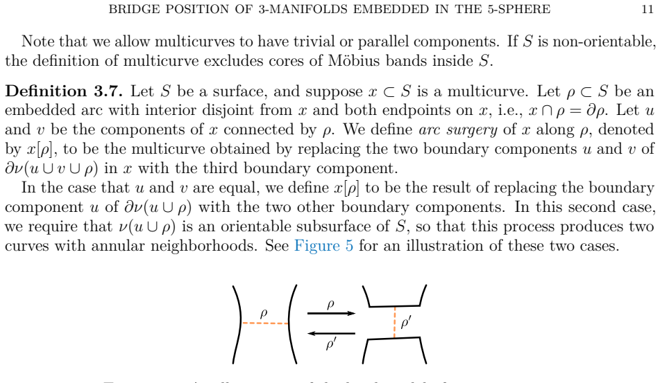
Figure 5. Figure 5: An illustration of the local model of an arc surgery. For example, in a pair of pants with boundaries u, v, and w, one can obtain w from u ∪ v by one arc surgery along a seam. One can interpret arc surgery as a 2-dimensional 1-handle attachment to ν(u ∪ v), and in particular, one arc surgery along ρ can be undone by arc surgery along the cocore of ν(ρ); see [PITH_FULL_IMAGE:figures/full_fig_p011_5.png] view at source ↗
Figure 6
Figure 6. Figure 6: Three local models for a perturbation of an abstract 4-section, where a, b, c and d correspond to the red, blue, green, and purple subgraphs. Top: an illustration of an a-perturbation. Middle: an illustration of an ab￾perturbation. Bottom: an illustration of an abc-perturbation. After each kind of local modification above, the result is clearly still an abstract 4-section. In fact, the simple closed curves… view at source ↗
Figure 7
Figure 7. Figure 7: An illustration of the proof of Lemma 3.12. By performing repeated perturbations along an arc, we can find a new abstract 4-section which realizes arc surgery of Γac along ρ. Once |int(ρ) ∩ Γbd| = 1, we proceed as in the previous case. □ Example 3.13. We illustrate the previous process with an example [PITH_FULL_IMAGE:figures/full_fig_p013_7.png] view at source ↗
Figure 8
Figure 8. Figure 8: An illustration of a sequence of arc surgeries on an abstract 4- section of the torus. Each arc surgery is indicated by a dashed arrow. The process converts Γac from two copies of the (0, 1) curve to two copies of the (0, 1) curve [PITH_FULL_IMAGE:figures/full_fig_p013_8.png] view at source ↗
Figure 9
Figure 9. Figure 9: An illustration of a sequence of arc surgeries on an abstract 4- section of the torus. Each arc surgery is indicated by a dashed arrow. In this case, the process converts Γac from two copies of the (0, 1) curve to two copies of the (2, 1) curve. 3.3. Perturbations of both abstract and embedded surfaces. Let T = (T1, T2, T3, T4) be a bridge 4-section of an embedded surface Σ : S ,→ S 4 . If Γ is the spine o… view at source ↗
Figure 10
Figure 10. Figure 10: Left: a schematic Heegaard complex of S 3 ⊂ S 5 , notice that all the data in the Heegaard complex is actually embedded in 3-space. Right: a depiction of the intersection of S 3 with the four sectors of the genus-zero 4-section of S 5 . Note that the disks Dα and Dβ, shaded in the figure, lie in the cross-section 3-spheres obtained by gluing two 3-balls. (1) ∂Dα = T1 ∪ T3, and (2) ∂Dβ = T2 ∪ T4. Proof. By… view at source ↗
Figure 11
Figure 11. Figure 11: Quadrisecting the 5-sphere [PITH_FULL_IMAGE:figures/full_fig_p019_11.png] view at source ↗
Figure 12
Figure 12. Figure 12: Treating a triple of crossingless tangles as a trisection, it is possible to cap off with trivial disk systems to form a closed surface, which is a trivial link of 2-spheres. Since the surface-link is trivial, we can fill in with a collection of 3-balls, which a priori lies in the union of the 3 balls Z12 ∪ Z13 ∪ Z24 ∪ Z34. The intersection B3 123 with Z24 ∪ Z34 is a collection of 3-balls that trace an is… view at source ↗
Figure 13
Figure 13. Figure 13: Left: an abstract 4-section of a torus. The blue-purple curves are meridians while the red-green have slope p/1. Middle: a bridge 4-sected embedding of the lens space L(p, 1) in S 5 , p ≥ 1. Right: the particular case p = 3. this for the p = 3 case and leave it as an exercise for the reader to generalize the figures for arbitrary p ≥ 2 [PITH_FULL_IMAGE:figures/full_fig_p023_13.png] view at source ↗
Figure 14
Figure 14. Figure 14: The tangles (T1, T2, T3, T4) from [PITH_FULL_IMAGE:figures/full_fig_p024_14.png] view at source ↗
Figure 15
Figure 15. Figure 15: The tangles (T1, T2, T3, T4) from [PITH_FULL_IMAGE:figures/full_fig_p024_15.png] view at source ↗
Figure 16
Figure 16. Figure 16: Left: a Heegaard diagram (Σ; α, β) of the 3-torus. Note that, looking at the way Σ is drawn in R 3 , each curve bounds a compressing disk for Σ embedded in R 3 . Thus, we have a Heegaard complex for a 3-torus in R 4 = R 3 ×R. Middle: doubling each curve in α∪β yields an abstract 4-section for Σ. This is drawn so that all the punctures lie in the same plane P ⊂ R 3 ; the rest of Σ and the arcs lie behind P… view at source ↗
Figure 17
Figure 17. Figure 17: Consider the tangles (T1, T2, T3, T4) from [PITH_FULL_IMAGE:figures/full_fig_p026_17.png] view at source ↗
Figure 18
Figure 18. Figure 18: Top: each panel is a local picture of a boundary parallel disk of F ∩ Xi+1 near the boundary ∂Xi+1. Sequences (A) and (B) depict an isotopy of the yellow surface in S 4 obtained by sliding the boundary of the surface through the trivial disk F ∩ Xi+1. Bottom: the effect of this isotopy is to trade a bridge disk for the red tangle with a combination of spanning surfaces for the red and blue tangles. T as i… view at source ↗
Figure 19
Figure 19. Figure 19: In (B)-(E): a sequence of perturbations of a bridge 4-sected surface in a neighborhood of a 1-bridge unknotted component of T2 ∪ T4. The effect of this sequence, shown in panel (E), is a new 1-bridge unknotted component of T1 ∪ T3 that appears with the property that the disk it bounds is isotopic in S 4 to the 4-bridge unknotted component of T2 ∪ T4. See Lemma 6.3. 1-bridge unknots as in (B) often appear … view at source ↗
Figure 20
Figure 20. Figure 20: Sequence of isotopies of the gray shaded disk in the left panel using the modifications in Remark 6.2 and [PITH_FULL_IMAGE:figures/full_fig_p029_20.png] view at source ↗
Figure 21
Figure 21. Figure 21: Alternative sequence of detubings and deperturbations transform￾ing the 4-plane diagram in [PITH_FULL_IMAGE:figures/full_fig_p030_21.png] view at source ↗
Figure 22
Figure 22. Figure 22: After removing the purple tangle from T2 in [PITH_FULL_IMAGE:figures/full_fig_p031_22.png] view at source ↗
Figure 23
Figure 23. Figure 23: Left: a 4-plane diagram for the ribbon 2-knot FKT . The shaded regions depict the meridian of the tube that undoes FKT . Right: the spine of a bridge 4-section of the 3-knot D(FKT ); see Example 6.5. 6.3. Spun 3-manifolds. Spinning is a process for building knotted objects from knots in lower dimensions, initiated by Artin a century ago [Art25]. To build 3-knots in S 5 , we can spin knots in either S 3 or… view at source ↗
Figure 24
Figure 24. Figure 24: In (A): a plat projection of a link K ⊂ S 3 . In (B): a quadrisection diagram for S 2 (K) ⊂ S 5 . Proposition 6.7. Let K ⊂ S 3 be a b-bridge knot or link. Then S 2 (K) admits a (5b−4)-bridge quadrisection with spine described in [PITH_FULL_IMAGE:figures/full_fig_p032_24.png] view at source ↗
Figure 25
Figure 25. Figure 25: The critical values of the function π |S2(K) . The preimage of every red ray is equal to the red tangle K◦ . The purple rays lie in a plane x3 = 1.5 and are based in the x3-axis; their preimage under h is the purple tangle K◦ 1.5 shown in the middle panel. The movie from 0 to ∞ is the same as from 0 to −∞. As r goes from −∞ to −1.5, we see two births. As t goes from −1.5 to 0, the two endpoints of K◦ r co… view at source ↗
Figure 26
Figure 26. Figure 26: In (A): a banded unlink diagram, and in (C): a 4-plane diagram representing the surface S 2 (K) ∩ R 4 −1.5 , obtained by spinning the tangle K◦ −1.5 along its boundary. In (B): a banded unlink diagram and, in (D): a 4-plane diagram representing S 2 (K) ∩ R 4 0 , equal to the spin of K. These two surfaces differ by a 1-handle addition shown. In (D): a Heegaard complex for S 2 -spun of K; the disk sets Dα =… view at source ↗
Figure 27
Figure 27. Figure 27: An illustration of S 2 × S 3 as a 2-fold cover of S 5 branched along an unknotted S 1 × S 2 . Left: a genus-two 4-section diagram as a 2-fold cover of a 2-phere branched along eight points. Middle: the colored curves descend to arcs, which correspond to a tuple of trivial tangles (T1, T2, T3, T4) shown in the middle panel. Right: embedding the graph T1 ∪ T2 ∪ T3 ∪ T4 in a torus. From Proposition 2.7, we s… view at source ↗
Figure 28
Figure 28. Figure 28: Consider a bridge quadrisection (S 5 , Y 3 ) = S4 i=1(Wi , Ei). The labeling convention in Definition 2.5 yields a hypercube of epimorphisms determined by tuples of homomorphisms (in black) from the fundamental group of a 2b-punctured surface to the fundamental group of tangle complements Bi \ Ti . Left and right diagrams correspond to the group quadrisection and group trisection for π1(S 5 \ Y 3 ) and π1… view at source ↗
read the original abstract

We introduce and study bridge decompositions for 3-manifolds embedded in the 5-sphere. These generalize both the classical notion of bridge position for knots in the 3-sphere and the bridge trisections of surfaces in the 4-sphere due to Meier and Zupan. Our main technical tool is the multisections of 5-manifolds introduced by Aribi, Courte, Golla, and Moussard. We prove that every embedded 3-manifold admits such a decomposition; in particular, any such embedding is encoded by four trivial tangle diagrams. We also present a range of explicit examples, including $S^2$-spun knots and ribbon 3-knots.

Editorial analysis

A structured set of objections, weighed in public.

Desk editor's note, referee report, simulated authors' rebuttal, and a circularity audit. Tearing a paper down is the easy half of reading it; the pith above is the substance, this is the friction.

Referee Report

2 major / 2 minor

Summary. The paper introduces bridge decompositions for 3-manifolds embedded in the 5-sphere, generalizing classical bridge positions for knots in S^3 and bridge trisections for surfaces in S^4. Employing multisections of 5-manifolds from prior work, it proves that every such embedded 3-manifold admits a decomposition into four trivial tangles, thereby encoding any embedding via four trivial tangle diagrams. Explicit examples are given, including S^2-spun knots and ribbon 3-knots.

Significance. If the central existence result holds, the work supplies a diagrammatic encoding for codimension-2 embeddings of 3-manifolds in S^5, extending lower-dimensional techniques in a natural way. The reliance on established multisection technology is a methodological strength, and the concrete examples demonstrate immediate applicability to spun and ribbon constructions. This framework may support further classification efforts or invariants in higher-dimensional knot theory.

major comments (2)
  1. The proof of the main existence theorem (the claim that every embedding admits a bridge decomposition into four trivial tangles) depends on isotoping an arbitrary 3-manifold embedding to meet a standard multisection of S^5 in trivial 4-tangles. The manuscript should supply a more detailed general-position argument establishing that such an isotopy always exists and preserves the embedding type, especially for knotted or non-separating cases where non-trivial intersections might persist.
  2. In the definition of the bridge decomposition and the encoding statement, clarify precisely how the four trivial tangle diagrams, together with the multisection data, determine the 3-manifold and its embedding in S^5 up to isotopy; any additional gluing or sector information required should be stated explicitly.
minor comments (2)
  1. In the abstract, briefly indicate the number of sectors in the multisection or the dimension of the tangles to give readers immediate context for the four-diagram encoding.
  2. For the examples of S^2-spun knots, consider adding a schematic diagram of the corresponding trivial tangle diagrams to improve visual clarity and accessibility.

Simulated Author's Rebuttal

2 responses · 0 unresolved

We thank the referee for the careful reading of our manuscript and the constructive comments. We address each major point below and will incorporate revisions to strengthen the exposition of the main theorem and the encoding statement.

read point-by-point responses
  1. Referee: The proof of the main existence theorem (the claim that every embedding admits a bridge decomposition into four trivial tangles) depends on isotoping an arbitrary 3-manifold embedding to meet a standard multisection of S^5 in trivial 4-tangles. The manuscript should supply a more detailed general-position argument establishing that such an isotopy always exists and preserves the embedding type, especially for knotted or non-separating cases where non-trivial intersections might persist.

    Authors: We agree that the general-position argument underlying the isotopy in the proof of the main existence result (Theorem 1.1) would benefit from greater detail. The current argument relies on standard transversality techniques for embeddings in high-dimensional manifolds, combined with the multisection framework of Aribi–Courte–Golla–Moussard, but we acknowledge that explicit control over intersections in knotted or non-separating cases is not spelled out at the level of individual steps. In the revised manuscript we will expand the relevant paragraph in Section 3 to include a self-contained sequence of isotopies: first making the 3-manifold transverse to the multisection hypersurfaces, then using dimension counts to eliminate non-trivial intersections while preserving the embedding type, with separate subcases for separating and non-separating components. revision: yes

  2. Referee: In the definition of the bridge decomposition and the encoding statement, clarify precisely how the four trivial tangle diagrams, together with the multisection data, determine the 3-manifold and its embedding in S^5 up to isotopy; any additional gluing or sector information required should be stated explicitly.

    Authors: We accept that the encoding statement in the introduction and in Definition 2.3 could be stated more explicitly. The four trivial tangle diagrams, together with the fixed standard multisection of S^5 (including the three 4-dimensional sectors and their pairwise intersections), determine the embedded 3-manifold up to isotopy once the gluing maps between the sectors are specified; these maps are induced by the standard identification of the boundary 3-spheres. In the revision we will add a short paragraph immediately after Definition 2.3 that lists the complete data set (four diagrams plus the sector gluing diffeomorphisms) and explains how the 3-manifold and its embedding are reconstructed by gluing the four trivial 4-tangles along these maps. revision: yes

Circularity Check

0 steps flagged

No circularity: central existence result applies external multisection technology to new setting

full rationale

The paper proves that every embedded 3-manifold in S^5 admits a bridge decomposition into four trivial tangles by intersecting the embedding with a multisection of the 5-sphere whose sectors are standard balls. This multisection technology is taken directly from the independent prior work of Aribi–Courte–Golla–Moussard (different authors) and is not derived or redefined within the present manuscript. The subsequent isotopy step that renders the intersections trivial tangles is a new application rather than a self-referential fit, renaming, or ansatz smuggled via self-citation. No equations reduce to their own inputs by construction, no uniqueness theorem is imported from the authors' prior work, and the argument remains self-contained against the external benchmark of the cited multisection existence result. The derivation therefore carries no load-bearing circularity.

Axiom & Free-Parameter Ledger

0 free parameters · 1 axioms · 0 invented entities

The central claim rests on the existence and applicability of multisections from prior work, with no free parameters, new entities, or ad-hoc axioms introduced in the abstract.

axioms (1)
  • domain assumption Multisections of 5-manifolds as defined and studied by Aribi, Courte, Golla, and Moussard exist and support the required decompositions.
    Invoked as the main technical tool for proving the bridge decomposition.

pith-pipeline@v0.9.0 · 5431 in / 1138 out tokens · 61841 ms · 2026-05-10T16:19:18.912377+00:00 · methodology

discussion (0)

Sign in with ORCID, Apple, or X to comment. Anyone can read and Pith papers without signing in.

Reference graph

Works this paper leans on

3 extracted references · 3 canonical work pages

  1. [1]

    Group trisections and smooth4- manifolds

    [AGK18] Aaron Abrams, David Gay, and Robion Kirby. “Group trisections and smooth4- manifolds.”Geometry & Topology22.3 (2018), pp. 1537–1545 (↑36). [AF21] Ian Agol and Michael Freedman. “Embedding Heegaard decompositions.”New Zealand Journal of Mathematics52 (2021), pp. 727–731 (↑24). [Ale20] James W. Alexander. “Note on Riemann spaces.”Bulletin of the Ame...

  2. [2]

    Knot spinning

    Encyclopaedia of Mathematical Sciences. Low-Dimensional Topology, III. Springer- Verlag, Berlin, 2004, pp. xiv+213 (↑9). [Cou+26] Sylvain Courte, Delphine Moussard, Qiuyu Ren, and Xiaozhou Zhou.Private communi- cation. Jan. 2026 (↑3). [Fri05] Greg Friedman. “Knot spinning.”Handbook of Knot Theory. Elsevier B. V., Amsterdam, 2005, pp. 187–208 (↑31). [GK16]...

  3. [3]

    Bridge trisections of knotted surfaces inS4

    Contemporary Mathematics. American Mathe- matical Society, Providence, RI, 1983, pp. 249–270 (↑2, 37, 38). [MMZ26] Jeffery Meier, Delphine Moussard, and Alexander Zupan.Private communication. Jan. 2026 (↑21). [MZ17] Jeffrey Meier and Alexander Zupan. “Bridge trisections of knotted surfaces inS4.” Transactions of the American Mathematical Society369.10 (20...