Towards a Robust Estimate of the Solar Photospheric Poynting Flux and Helicity Flux
Pith reviewed 2026-05-10 07:33 UTC · model grok-4.3
The pith
Differences in Doppler velocity handling cause major discrepancies in estimates of solar Poynting and helicity fluxes.
A machine-rendered reading of the paper's core claim, the machinery that carries it, and where it could break.
Core claim
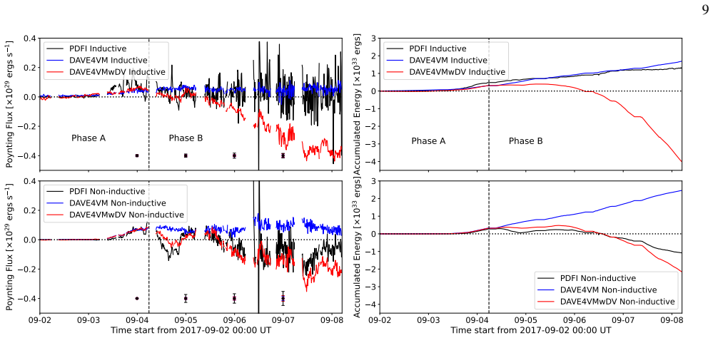
On NOAA active region 12673, the PDFI, DAVE4VM, and DAVE4VMwDV methods yield inconsistent accumulated Poynting and helicity fluxes. The Helmholtz-Hodge decomposition demonstrates that Doppler velocities significantly influence the non-inductive electric field contribution to these fluxes, and the ad hoc treatments of velocities in the methods account for the observed differences in values and signs.
What carries the argument
Helmholtz-Hodge decomposition of the observed velocity field to separate contributions to the electric field, highlighting the role of the non-inductive component from Doppler velocity.
If this is right
- Improved velocity observations are required to better constrain the electric field estimates.
- Standardizing the treatment of Doppler and transverse velocities across methods would reduce inconsistencies in flux calculations.
- The choice of method affects conclusions about energy and helicity injection in active regions.
- Future work should focus on observations that minimize uncertainties in velocity components.
Where Pith is reading between the lines
- These discrepancies could impact models of solar flare and coronal mass ejection triggering that rely on photospheric flux inputs.
- Applying the decomposition to other active regions might reveal if the Doppler contribution is generally significant.
- Simulations with known ground-truth velocities could test which method recovers the true fluxes most accurately.
Load-bearing premise
The Helmholtz-Hodge decomposition cleanly separates the inductive and non-inductive electric field contributions from the observed velocities without substantial interference from measurement errors or the particular properties of the active region.
What would settle it
High-precision, simultaneous measurements of all velocity components in a well-observed active region where independent verification of the total energy input is possible, or controlled numerical simulations where the true Poynting flux is known.
Figures


read the original abstract
The observed solar photospheric magnetic fields and Doppler velocities are frequently used to quantify the Poynting flux and helicity flux. Multiple methods have been developed for this purpose, but their estimates of the Poynting flux and helicity flux often differ from one another. Here we study the performance of three widely used methods on NOAA active region 12673: "PTD-Doppler-FLCT Ideal" (PDFI), "Differential Affine Velocity Estimator for Vector Magnetograms" (DAVE4VM), and an extension of the latter with Doppler velocity constraint (DAVE4VMwDV). We find that the values of the accumulated energy and helicity differ significantly between the three methods, even in signs. Using the Helmholtz-Hodge decomposition, we show that Doppler velocity can contribute significantly to the Poynting flux and helicity flux through the non-inductive (curl-free) electric field. The different, ad hoc treatments of the Doppler and transverse velocities in three methods are directly responsible for the discrepancies. We discuss the desired future observations that can better constrain these methods.
Editorial analysis
A structured set of objections, weighed in public.
Referee Report
Summary. The manuscript compares three methods (PDFI, DAVE4VM, and DAVE4VMwDV) for computing photospheric Poynting and helicity fluxes from vector magnetograms and Doppler velocities observed in NOAA AR 12673. It reports large differences in accumulated energy and helicity (including sign reversals) across the methods and applies the Helmholtz-Hodge decomposition to the velocity fields to show that Doppler velocities contribute substantially to the fluxes through the curl-free (non-inductive) electric-field component. The central claim is that the discrepancies originate directly from the differing, ad-hoc treatments of Doppler versus transverse velocities in the three algorithms.
Significance. If the attribution holds, the work is significant because Poynting and helicity fluxes are central inputs to models of coronal heating and eruptive activity; clarifying why standard methods disagree improves the reliability of these quantities. The explicit use of Helmholtz-Hodge decomposition on real data provides a useful diagnostic that can guide future algorithm development. The analysis is grounded in a well-observed active region and employs existing, widely used velocity estimators rather than introducing new free parameters.
major comments (2)
- [Helmholtz-Hodge decomposition analysis (results section)] The attribution of all sign and magnitude discrepancies to velocity-handling differences rests on the Helmholtz-Hodge decomposition isolating a substantial non-inductive contribution from the Doppler velocities. However, the manuscript provides no error propagation through the decomposition, no synthetic-data tests with controlled noise levels (typical photospheric Doppler uncertainties are several hundred m/s), and no assessment of leakage from measurement noise or AR-specific flows into the curl-free component. This leaves the isolation unverified and weakens the claim that velocity-treatment differences are the sole or primary cause.
- [Method comparison and accumulated-flux results] The quantitative comparison of accumulated energy and helicity across the three methods does not include a controlled isolation of the effect of each velocity constraint (e.g., the Doppler constraint added in DAVE4VMwDV versus the unconstrained DAVE4VM). Without such a breakdown or sensitivity runs that vary only the Doppler/transverse handling while holding other algorithmic assumptions fixed, it remains unclear how much of the reported discrepancy is truly due to the ad-hoc treatments versus other differences in electric-field reconstruction.
minor comments (2)
- [Abstract] The abstract states that the methods 'differ significantly' but does not report the actual numerical values or ratios of the accumulated fluxes, making it harder for readers to gauge the practical size of the discrepancies.
- [Figures and methods section] Figure captions and the data-processing description lack explicit statements of the spatial and temporal resolution, the exact time interval used for accumulation, and whether any smoothing or interpolation was applied to the velocity fields before decomposition.
Simulated Author's Rebuttal
We thank the referee for the constructive and detailed review of our manuscript. The comments highlight important aspects of the analysis that we will address in the revision. We respond to each major comment below.
read point-by-point responses
-
Referee: [Helmholtz-Hodge decomposition analysis (results section)] The attribution of all sign and magnitude discrepancies to velocity-handling differences rests on the Helmholtz-Hodge decomposition isolating a substantial non-inductive contribution from the Doppler velocities. However, the manuscript provides no error propagation through the decomposition, no synthetic-data tests with controlled noise levels (typical photospheric Doppler uncertainties are several hundred m/s), and no assessment of leakage from measurement noise or AR-specific flows into the curl-free component. This leaves the isolation unverified and weakens the claim that velocity-treatment differences are the sole or primary cause.
Authors: We acknowledge that the manuscript does not include formal error propagation through the Helmholtz-Hodge decomposition or synthetic tests with controlled noise levels. The decomposition is applied directly to the velocity fields derived from the three methods on the observed data of NOAA AR 12673 to illustrate that the curl-free (non-inductive) component associated with Doppler velocities contributes substantially to both the Poynting and helicity fluxes. This provides a diagnostic explanation for the sign and magnitude differences seen in the accumulated quantities. We agree, however, that the robustness of this isolation against typical Doppler uncertainties and possible leakage has not been quantified. In the revised manuscript we will add a dedicated discussion of these limitations together with a set of synthetic tests that inject controlled noise levels into the velocity fields before decomposition. revision: yes
-
Referee: [Method comparison and accumulated-flux results] The quantitative comparison of accumulated energy and helicity across the three methods does not include a controlled isolation of the effect of each velocity constraint (e.g., the Doppler constraint added in DAVE4VMwDV versus the unconstrained DAVE4VM). Without such a breakdown or sensitivity runs that vary only the Doppler/transverse handling while holding other algorithmic assumptions fixed, it remains unclear how much of the reported discrepancy is truly due to the ad-hoc treatments versus other differences in electric-field reconstruction.
Authors: We note that DAVE4VM and DAVE4VMwDV share the same core differential affine velocity estimator and differ only in the explicit inclusion of the Doppler velocity constraint; their direct comparison therefore isolates the effect of that constraint. PDFI, by contrast, employs an independent Poloidal-Toroidal decomposition that incorporates both Doppler and FLCT transverse velocities under different assumptions. Nevertheless, we agree that an explicit breakdown or additional sensitivity experiments that vary only the Doppler/transverse handling while freezing other algorithmic choices would make the attribution clearer. We will add such a controlled comparison and sensitivity analysis to the revised manuscript. revision: yes
Circularity Check
No significant circularity; analysis is empirical comparison on observational data
full rationale
The paper applies three established velocity-inversion methods (PDFI, DAVE4VM, DAVE4VMwDV) and the standard Helmholtz-Hodge decomposition directly to vector magnetogram and Doppler data from NOAA 12673. Discrepancies in accumulated Poynting and helicity fluxes are shown by explicit numerical evaluation on the same input observations; no parameter is fitted to a subset and then relabeled as a prediction, no equation reduces by construction to its own input, and no load-bearing premise rests on a self-citation chain. The derivation chain is therefore self-contained against external benchmarks and receives the default non-circularity finding.
Axiom & Free-Parameter Ledger
axioms (1)
- domain assumption The Helmholtz-Hodge decomposition separates the electric field into inductive (curl) and non-inductive (curl-free) parts that can be computed from observed velocities and magnetic fields.
Reference graph
Works this paper leans on
-
[1]
, " * write output.state after.block = add.period write newline
ENTRY address archivePrefix author booktitle chapter doi edition editor eprint howpublished institution journal key month number organization pages publisher school series title misctitle type volume year version url label extra.label sort.label short.list INTEGERS output.state before.all mid.sentence after.sentence after.block FUNCTION init.state.consts ...
-
[2]
" write newline "" before.all 'output.state := FUNCTION format.url url empty "" new.block "" url * "" * if FUNCTION format.eprint eprint empty "" archivePrefix empty "" archivePrefix "arXiv" = new.block " " eprint * " " * new.block " " eprint * " " * if if if FUNCTION format.doi doi empty "" " " doi * " " * if FUNCTION format.pid doi empty eprint empty ur...
-
[3]
- [1] #1 = = ^ ^ ^ .\!\!^ d .\!\!^ h .\!\!^ m .\!\!^ s .\!\!^ @mss
thebibliography [1] 20pt to REFERENCES 6pt =0pt -12pt 10pt plus 3pt =0pt =0pt =1pt plus 1pt =0pt =0pt -12pt =13pt plus 1pt =20pt =13pt plus 1pt \@M =10000 =-1.0em =0pt =0pt 0pt =0pt =1.0em @enumiv\@empty 10000 10000 `\.\@m \@noitemerr \@latex@warning Empty `thebibliography' environment \@ifnextchar \@reference \@latexerr Missing key on reference command E...
discussion (0)
Sign in with ORCID, Apple, or X to comment. Anyone can read and Pith papers without signing in.