ML, PL, QL in Markov chain models
Pith reviewed 2026-05-09 23:24 UTC · model grok-4.3
The pith
Quasi-likelihood matches full maximum likelihood closely while gaining robustness over pseudo-likelihood in Markov chain models.
A machine-rendered reading of the paper's core claim, the machinery that carries it, and where it could break.
Core claim
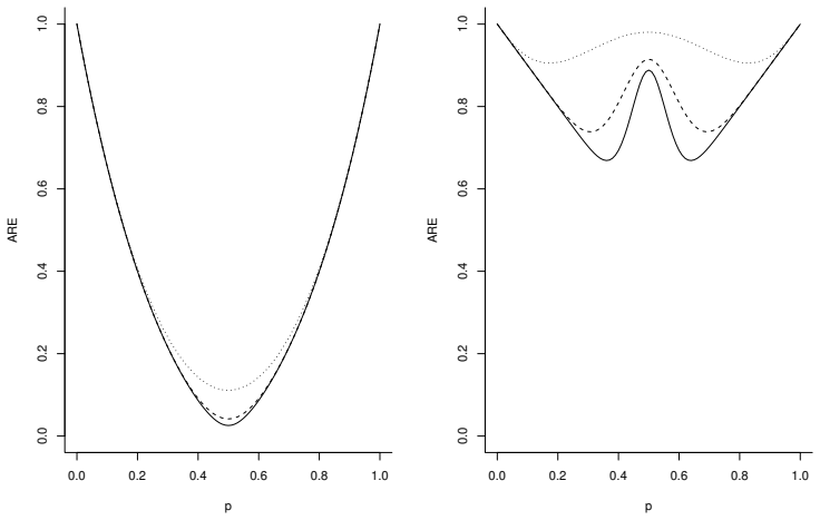
The paper derives limiting normality results for the maximum likelihood, pseudo-likelihood, and quasi-likelihood estimators in general Markov chain models. It shows that the quasi-likelihood strategy is typically preferable to the pseudo-likelihood, losing very little to the maximum likelihood while gaining in model robustness, and has potential as a modelling tool.
What carries the argument
Limiting normality results for the three estimators, with pseudo-likelihood and quasi-likelihood treated as maximum penalised likelihood methods.
If this is right
- Quasi-likelihood becomes a practical substitute when full maximum likelihood is computationally prohibitive due to complex dependencies.
- Quasi-likelihood retains most efficiency of full maximum likelihood across the examined Markov settings.
- Pseudo-likelihood shows consistent efficiency losses relative to the other two methods.
- The methods apply directly to spatial-temporal and DNA sequence models.
Where Pith is reading between the lines
- Quasi-likelihood could be implemented as a default option in software for dependent data analysis when full likelihood is intractable.
- The robustness advantage might prove useful in spatial models where the exact dependence structure is uncertain.
- Finite-sample checks on non-DNA Markov chains would test whether the asymptotic preference for quasi-likelihood holds in practice.
Load-bearing premise
The limiting normality results accurately capture finite-sample behavior and the performance comparisons extend beyond the DNA sequence examples considered.
What would settle it
A simulation study on finite-length Markov chains with known parameters, comparing the three estimators' bias, variance, and robustness under model misspecification, would confirm or refute the asymptotic rankings.
Figures


read the original abstract
In many spatial and spatial-temporal models, and more generally in models with complex dependencies, it may be too difficult to carry out full maximum likelihood (ML) analysis. Remedies include the use of pseudo-likelihood (PL) and quasi-likelihood (QL) (also called the composite likelihood). The present article studies the ML, the PL and the QL methods for general Markov chain models, partly motivated by the desire to understand the precise behaviour of PL and QL methods in settings where this can be analysed. We present limiting normality results and compare performances in different settings. The PL and QL methods can be seen as maximum penalised likelihood methods. We find that the QL strategy is typically preferable to the PL, and that it loses very little to the ML, while earning in model robustness. It has also appeal and potential as a modelling tool. Our methods are illustrated for analysis of DNA sequence evolution type models.
Editorial analysis
A structured set of objections, weighed in public.
Referee Report
Summary. The paper derives limiting normality results for maximum likelihood (ML), pseudo-likelihood (PL), and quasi-likelihood (QL) estimators in general Markov chain models. It compares their asymptotic efficiencies and finite-sample performance on DNA sequence evolution examples, concluding that QL is typically preferable to PL (losing little to ML while gaining robustness) and has appeal as a modeling tool.
Significance. If the derivations and comparisons hold, the work provides useful theoretical grounding and practical guidance for choosing among ML, PL, and QL in dependent-data settings where full likelihood is intractable. The explicit limiting normality results and the framing of PL/QL as penalized likelihood are strengths that allow precise efficiency comparisons.
major comments (2)
- [Performance comparisons and illustrations] The headline claim that QL is 'typically preferable' to PL (while close to ML) rests on the limiting normality results plus DNA-sequence illustrations. These are asymptotic; without finite-sample simulations across a range of chain lengths, orders, or transition structures, the finite-sample preference and robustness advantage do not necessarily follow (see stress-test concern).
- [Robustness discussion] The robustness advantage of QL is asserted but not quantified beyond the DNA examples. A concrete measure (e.g., sensitivity to misspecification of the transition kernel or to higher-order dependence) would be needed to support the general claim that QL 'earns in model robustness.'
minor comments (2)
- [Methods] Notation for the composite likelihood and the penalization terms could be clarified with an explicit equation early in the methods section.
- [Abstract] The abstract states 'limiting normality results' but does not indicate whether the results cover both stationary and non-stationary chains; a brief statement would help readers.
Simulated Author's Rebuttal
We thank the referee for the detailed and constructive report. The comments highlight opportunities to strengthen the finite-sample evidence supporting our claims. We address each major point below and will incorporate revisions to provide additional simulation-based support for the performance and robustness conclusions.
read point-by-point responses
-
Referee: [Performance comparisons and illustrations] The headline claim that QL is 'typically preferable' to PL (while close to ML) rests on the limiting normality results plus DNA-sequence illustrations. These are asymptotic; without finite-sample simulations across a range of chain lengths, orders, or transition structures, the finite-sample preference and robustness advantage do not necessarily follow (see stress-test concern).
Authors: We agree that the current finite-sample support relies on the DNA sequence illustrations in Section 5 rather than a broad Monte Carlo study. The limiting normality results (Theorems 3.1, 4.1, and 4.2) and the efficiency comparisons derived from them establish the asymptotic preference for QL over PL with minimal loss relative to ML. The DNA examples demonstrate this in a practical setting with finite lengths. To address the concern directly, we will add a new simulation subsection varying chain lengths (n = 50 to 2000), Markov orders (1 and 2), and transition probability structures, reporting empirical bias, variance, and coverage to confirm the finite-sample behavior aligns with the asymptotics. revision: yes
-
Referee: [Robustness discussion] The robustness advantage of QL is asserted but not quantified beyond the DNA examples. A concrete measure (e.g., sensitivity to misspecification of the transition kernel or to higher-order dependence) would be needed to support the general claim that QL 'earns in model robustness.'
Authors: The robustness claim follows from the construction of QL as a composite likelihood that depends only on the specified transition kernel (unlike full ML) and avoids the pairwise over-weighting issues of PL, as framed in Section 2. The DNA examples provide empirical illustration under potential model departures common in sequence data. We will add a targeted simulation study in the revision that generates data from a misspecified higher-order chain and fits first-order models, comparing mean squared error and robustness metrics (e.g., relative efficiency loss under misspecification) across ML, PL, and QL to quantify the advantage. revision: yes
Circularity Check
No significant circularity; derivations rely on standard asymptotic theory
full rationale
The paper derives limiting normality results for ML, PL and QL estimators in general Markov chain models from standard asymptotic theory for dependent processes. Efficiency comparisons and the conclusion that QL is typically preferable to PL follow directly from these limiting distributions and relative asymptotic variances, without any reduction to fitted parameters, self-definitions, or load-bearing self-citations. DNA sequence illustrations are presented as applications after the theory, not as the source of the claims. The derivation chain is self-contained against external benchmarks.
Axiom & Free-Parameter Ledger
axioms (1)
- domain assumption Markov chain models satisfy standard regularity conditions allowing central limit theorems for the estimators
Reference graph
Works this paper leans on
-
[1]
Anderson, T.W. and Goodman, L.A. (1957). Statistical inference about Markov chains. Annals of Mathematical Statistics28, 89–110
work page 1957
-
[2]
Barry, D. and Hartigan, J.A. (1987). Asynchronous distance between homologous DNA sequences.Biometrics43, 261–276. Basawa and Rao (1980).Statistical Inference for Stochastic Processes.Academic Press, London
work page 1987
-
[3]
Basharin, G.P., Langville, A.N. and Naumov, V.A. (2004). The life and work of A.A. Markov.Linear Algebra and its Applications386, 3–26
work page 2004
-
[4]
Besag, J. (1974). Spatial interaction and the statistical analysis of lattice systems (with discussion contributions).Journal of the Royal Statistical SocietyB 36, 192–236
work page 1974
-
[5]
Besag, J. (1975). Statistical analysis of non-lattice data.The Statistician24, 179–195
work page 1975
-
[6]
Besag, J. (1977). Some methods of statistical analysis for spatial data.Bulletin of the Institute of International Statistics47, 77–92
work page 1977
-
[7]
Blaisdell, B. E. (1985). A method for estimating from two aligned present day DNA sequences their ancestral composition and subsequent rates of composition and subse- quent rates of substitution, possibly different in the two lineages, corrected for multiple and parallel substitutions at the same site.Journal of Molecular Evolution22, 69–81. 32
work page 1985
-
[8]
Cox, D. R. and Reid, N. (2004). A note on pseudolikelihood constructed from marginal densities.Biometrika91, 729–737
work page 2004
-
[9]
(2003).Statistical Models.Cambridge University Press, Cambridge
Davison, A.C. (2003).Statistical Models.Cambridge University Press, Cambridge
work page 2003
-
[10]
(2002).Probability Models for DNA Sequence Evolution.Probability and Its
Durret, R. (2002).Probability Models for DNA Sequence Evolution.Probability and Its
work page 2002
-
[11]
Fearnhead, P. and Donnelly, P. (2002). Approximate likelihood methods for estimating local recombination rates.Journal of the Royal Statistical SocietyB 64, 657–680
work page 2002
-
[12]
Fokianos, K. and Kedem, B. (2003). Regression theory for categorical time series.Statis- tical Science18, 357–375
work page 2003
-
[13]
Glasbey, C.A. (2001). Non-linear autoregressive time series with multivariate Gaussian mixtures as marginal distributions.Applied Statistics50, 143–154
work page 2001
-
[14]
Heagerty, P.J. and Lele, S.R. (1998). A composite likelihood approach to binary spatial data.Journal of the American Statistical Association93, 1099–1111
work page 1998
-
[15]
Henderson, R. and Shimakura, S. (2003). A serially correlated gamma frailty model for longitudinal count data.Biometrika90, 355–366
work page 2003
-
[16]
Hjort, N.L. and Mohn, E. (1987). Topics in the statistical analysis of remotely sensed data [with discussion].Bulletins of the International Statistical Institute52(Proceedings of the ISI Meeting, Tokyo), 23–44
work page 1987
-
[17]
Hjort, N.L. and Omre, H. (1994). Topics in spatial statistics (with discussion contribu- tions).Scandinavian Journal of Statistics21, 289–357
work page 1994
-
[18]
Hjort, N.L. and Mostad, P. (1998). A quasi-likelihood method for estimating parameters in spatial covariance functions. Manuscript
work page 1998
-
[19]
Hobolth, A. and Jensen, J.L. (2005). Statistical inference in evolutionary models of DNA sequences via the EM algorithm. Research report No. 455, Department of Theoretical
work page 2005
-
[20]
(1995).Statistical Methods Applied in Meteorology.Cand
Homleid, M. (1995).Statistical Methods Applied in Meteorology.Cand. scient. thesis, Department of Mathematics, University of Oslo
work page 1995
-
[21]
Karlin, S. and Taylor, H.M. (1975).A First Course in Stochastic Processes.Academic
work page 1975
-
[22]
Kimura, M. (1980). A simple method for estimating evolutionary rates of base substi- tutions through comparative studies of nucleotide sequences.Journal of Molecular Evolution16, 111–120
work page 1980
-
[23]
Kimura, M. (1981). Estimation of evolutionary distances between homologous nucleotide sequences.Proceedings of the National Academy of Sciences USA78, 454–458. de Leon, A.R. (2004). Pairwise likelihood approach to grouped continuous model and its extension. Technical report, Department of Mathematics & Statistics, University of Calgary
work page 1981
-
[24]
Lindsay, B. (1988). Composite likelihood methods. InStatistical Inference for Stochastic Processes(ed. N.U. Prahbu), American Mathematical Society. 33
work page 1988
-
[25]
Markov, A.A. (1906). Rasprostranenie zakona bol~xih qisel na veliqiny, zavis wie drug ot druga.Izvesti Fiziko-matematiqeskogo obqestva pri Ka- zanskom universitete15(2- seri ), 124–156
work page 1906
-
[26]
Markov, A.A. (1913). Primer statistiqeskogo issledovani nad tekstom “Ev- geni Onegina”, ill striru wi˘i sv z~ ispytani˘i v cep~.Izvesti Aka- demii Nauk, Sankt-Peterburg7(6- seri ), 153–162
work page 1913
-
[27]
Nott, D.J. and Ryd´ en, T. (1999). Pairwise likelihood methods for inference in image models.Biometrika86, 661–676
work page 1999
-
[28]
Parner, E.T. (2001). A composite likelihood approach to multivariate survival data.Scan- dinavian Journal of Statistics28, 295–302
work page 2001
-
[29]
Pickard, D.K. (1987). Inference for discrete Markov fields: the simplest nontrivial case. Journal of the American Statistical Association82, 90–96
work page 1987
-
[30]
(1977).Eugene Onegin[translated by C.H
Pushkin, A.S. (1977).Eugene Onegin[translated by C.H. Johnston]. Penguin Clas- sics, London. There are various later reprints of essentially the same translation of Pushkin’s 1833 epic
work page 1977
-
[31]
Renard, D., Molenberghs, G. and Geys, H. (2004). A pairwise likelihood approach to estimation in multilevel probit models.Computational Statistics & Data Analysis 44, 649–667
work page 2004
-
[32]
Strauss, D. and Ikeda, M. (1990). Pseudolikelihood estimation for social networks.Journal of the American Statistical Association85, 204–212
work page 1990
-
[33]
Taylor, H.M. and Karlin, S. (1984).An Introduction to Stochastic Modeling.Academic
work page 1984
-
[34]
Varin, C., Høst, G. and Skare, Ø. (2005). Pairwise likelihood inference in spatial general- ized linear mixed models.Computational Statistics & Data Analysis, to appear. 34
work page 2005
discussion (0)
Sign in with ORCID, Apple, or X to comment. Anyone can read and Pith papers without signing in.