Modelling spatial heterogeneity in the effects of area-level covariates on income distributions using Bayesian nonparametric methods
Pith reviewed 2026-05-08 07:42 UTC · model grok-4.3
The pith
Income distributions across areas are modeled as mixtures of shared latent factor densities whose weights vary smoothly with space and covariates.
A machine-rendered reading of the paper's core claim, the machinery that carries it, and where it could break.
Core claim
The Normalised Latent Measure Factor Model with Covariates expresses a collection of related densities as finite mixtures of latent factor densities, where the mixture weights depend on spatial coordinates and area-level covariates; an adaptive Gibbs sampler determines the number of factors, and a rotation method aligns posterior draws across separate data sets.
What carries the argument
The Normalised Latent Measure Factor Model with Covariates (NLMFM-C), a Bayesian nonparametric mixture model in which each area-level density is a weighted combination of shared latent factor densities whose weights are functions of space and covariates.
If this is right
- The number of underlying latent income regimes is inferred automatically from the data without being fixed in advance.
- The latent factors align with distinct income levels that can be labeled low, medium, or high.
- Covariate effects on the full income distribution, including those of gender, race, and educational attainment, can be estimated separately for each area and compared across years.
- Posterior summaries remain comparable across different collections of areas after applying the rotation step.
Where Pith is reading between the lines
- The same structure could be used to forecast full income distributions for unsampled sub-areas by interpolating the spatially smooth weights.
- Policy analysis could target areas where a given covariate shifts the upper tail of the income distribution more than the mean.
- The framework extends directly to other right-skewed economic outcomes such as wealth or expenditure distributions.
Load-bearing premise
Income distributions in different areas can be represented as mixtures of a modest number of common latent factor distributions whose weights change smoothly with spatial location and covariate values.
What would settle it
The posterior number of latent factors grows without bound when the model is refit to successively larger collections of sub-areas, or the predicted income distributions for held-out sub-areas deviate substantially from the observed histograms.
Figures


read the original abstract
Understanding the how the distribution of an economic outcome, such as income, changes with respect to space and covariates is a key concern for policy makers. To address this, we develop a Bayesian nonparametric model, the Normalised Latent Measure Factor Model with Covariates (NLMFM-C), which expresses a large collection of related densities as mixtures of latent factor densities and allows for spatial and covariate effects. We propose an adaptive Gibbs sampler to automatically infer the number of latent factor distributions, and a rotation method to make posterior inference on different data sets comparable. We apply the NLMFM-C model to Public Use Microdata Sample (PUMS) data, focusing on income distributions for sub-areas of four U.S. states over to different years, 2016 and 2020. We show that the latent factor distributions can be interpreted by income level (e.g., low, medium, and high) and investigate the spatially- and time-changing impact of three covariates: gender, race and educational attainment.
Editorial analysis
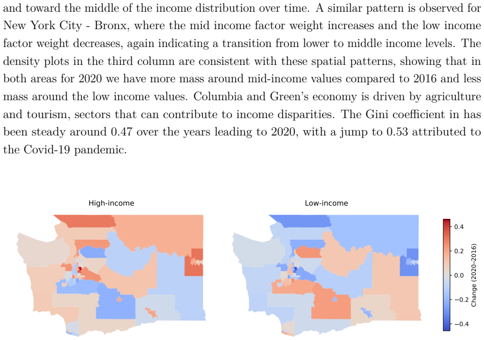
A structured set of objections, weighed in public.
Referee Report
Summary. The paper develops the Normalised Latent Measure Factor Model with Covariates (NLMFM-C), a Bayesian nonparametric model that represents collections of related income densities as mixtures of shared latent factor densities while incorporating spatial heterogeneity and covariate effects (gender, race, educational attainment). It introduces an adaptive Gibbs sampler to infer the number of latent factors and a rotation method to enable comparable posterior inference across datasets. The model is applied to PUMS income data from sub-areas of four U.S. states in 2016 and 2020, with latent factors interpreted as low-, medium-, and high-income components and analysis of spatially and temporally varying covariate impacts.
Significance. If the shared-factor mixture representation holds and the adaptive inference is reliable, the NLMFM-C would provide a flexible nonparametric framework for modeling spatial and covariate-driven heterogeneity in distributions, with interpretable latent components that could inform policy analysis in economics and spatial statistics. The automatic determination of model complexity via the Bayesian nonparametric construction and the rotation method for cross-year comparability are potential strengths that distinguish it from fixed-component alternatives.
major comments (3)
- [Model specification and inference (around the NLMFM-C definition)] The load-bearing assumption that income densities across areas are well-approximated by mixtures of a modest number of shared latent factor densities (with weights varying smoothly via the normalized latent measure) is not sufficiently validated. The adaptive Gibbs sampler selects the number of shared components but provides no diagnostics, residual analysis, or comparisons to area-specific mixture models to confirm that local features (e.g., distinct modes or heavy tails in sub-areas) are not misattributed to weight variation alone, which could bias the reported covariate effect estimates.
- [Application to PUMS data and results] The application section reports no quantitative goodness-of-fit metrics, posterior predictive checks, or baseline comparisons (e.g., independent per-area Dirichlet process mixtures or finite mixture models) for the PUMS data fits in 2016 and 2020. Without these, it is impossible to assess whether the shared latent factors adequately capture the observed distributions or whether the spatially- and time-varying effects of gender, race, and education are reliably estimated.
- [Inference and rotation method] The rotation method for cross-dataset comparability assumes stability of the learned latent factors across years, but no sensitivity analysis, perturbation checks, or assessment of factor stability under the nonparametric prior is provided. This is critical because the central claim of interpretable low/medium/high income factors and their covariate effects depends on this stability.
minor comments (2)
- [Abstract] The abstract contains a minor phrasing issue ('over to different years') that should be corrected for clarity.
- [Model development] Notation for the normalized latent measure construction and the covariate-dependent weights could be clarified with an explicit equation reference or diagram to aid readers unfamiliar with the construction.
Simulated Author's Rebuttal
We thank the referee for their constructive and detailed comments on our manuscript. These highlight key areas for strengthening the validation of the NLMFM-C model and its application. We address each major comment below and will make the indicated revisions to improve the paper.
read point-by-point responses
-
Referee: [Model specification and inference (around the NLMFM-C definition)] The load-bearing assumption that income densities across areas are well-approximated by mixtures of a modest number of shared latent factor densities (with weights varying smoothly via the normalized latent measure) is not sufficiently validated. The adaptive Gibbs sampler selects the number of shared components but provides no diagnostics, residual analysis, or comparisons to area-specific mixture models to confirm that local features (e.g., distinct modes or heavy tails in sub-areas) are not misattributed to weight variation alone, which could bias the reported covariate effect estimates.
Authors: We acknowledge that the current manuscript lacks explicit diagnostics to validate the shared latent factor assumption. In the revised version, we will add posterior predictive checks by simulating replicated income distributions from the fitted NLMFM-C posterior and comparing them visually and quantitatively (e.g., via integrated squared error or quantile differences) to the observed densities in representative sub-areas. We will also fit independent per-area Dirichlet process mixture models as a baseline and compare the resulting component counts, density shapes, and fit quality to assess whether local features such as modes or tails are adequately captured by weight variation on the shared factors alone. These additions will help confirm that the reported covariate effects are not biased by model misspecification. revision: yes
-
Referee: [Application to PUMS data and results] The application section reports no quantitative goodness-of-fit metrics, posterior predictive checks, or baseline comparisons (e.g., independent per-area Dirichlet process mixtures or finite mixture models) for the PUMS data fits in 2016 and 2020. Without these, it is impossible to assess whether the shared latent factors adequately capture the observed distributions or whether the spatially- and time-varying effects of gender, race, and education are reliably estimated.
Authors: We agree that the absence of quantitative fit assessments limits the evaluation of the results. In the revision, we will expand the application section to include posterior predictive checks for both the 2016 and 2020 PUMS datasets, reporting comparisons of key statistics such as means, variances, and tail probabilities between observed and replicated data. We will also add baseline comparisons by fitting independent per-area finite mixture models and Dirichlet process mixtures, using metrics like average log predictive density and Wasserstein distance between fitted and empirical distributions. These will be presented alongside the existing results to demonstrate the adequacy of the shared factors and the reliability of the spatially and temporally varying covariate effects. revision: yes
-
Referee: [Inference and rotation method] The rotation method for cross-dataset comparability assumes stability of the learned latent factors across years, but no sensitivity analysis, perturbation checks, or assessment of factor stability under the nonparametric prior is provided. This is critical because the central claim of interpretable low/medium/high income factors and their covariate effects depends on this stability.
Authors: The rotation method is designed to align comparable latent factors across years for consistent interpretation. We recognize the need to demonstrate its robustness. In the revised manuscript, we will include a sensitivity analysis by re-fitting the model to perturbed versions of the data (e.g., with small additive noise to income values or random subsampling of areas) and checking the stability of the identified low-, medium-, and high-income factor locations and shapes. We will also examine posterior variability in the factor parameters under the nonparametric prior and report how the interpretability and associated covariate effect estimates hold across these checks. This will strengthen the support for the cross-year comparability claims. revision: yes
Circularity Check
No circularity in NLMFM-C model derivation or inference
full rationale
The paper presents NLMFM-C as a new Bayesian nonparametric construction that represents area-level income densities via mixtures of shared latent factor densities, with weights modulated by spatial and covariate effects through a normalized latent measure. The adaptive Gibbs sampler infers the number of factors directly from the data, and the rotation method is a post-processing step for cross-dataset comparability; neither reduces any claimed prediction to a fitted parameter by construction. No load-bearing steps rely on self-citations, uniqueness theorems imported from prior author work, or ansatzes smuggled via citation. The derivation chain is self-contained: the model is defined, the sampler is specified, and results are obtained by fitting to PUMS data with post-hoc interpretation of factors. This is the standard case of an independent modeling contribution.
Axiom & Free-Parameter Ledger
free parameters (1)
- number of latent factors
axioms (2)
- domain assumption A collection of related densities can be expressed as mixtures of shared latent factor densities
- domain assumption Spatial and covariate effects can be incorporated by modulating the mixture weights
invented entities (1)
-
latent factor distributions
no independent evidence
Reference graph
Works this paper leans on
-
[1]
Federal Reserve Bank of San Francisco
URL https://www.clevelandfed.org/collections/press-releases/2025/ pr-20250331-demand-for-college-educated-workers-is-no-longer-growing-faster-than-supply . Federal Reserve Bank of San Francisco. Falling college wage premiums by race and ethnicity. FRBSF Economic Letter,
work page 2025
-
[2]
URL https://www. frbsf.org/research-and-insights/publications/economic-letter/2023/08/ falling-college-wage-premiums-by-race-and-ethnicity/. 27 T. S. Ferguson. A Bayesian analysis of some nonparametric problems.The Annals of Statistics, 1:209–230,
work page 2023
-
[3]
K. L. McKinney, J. M. Abowd, and H. P. Janicki. US long-term earnings outcomes by sex, race, ethnicity, and place of birth.Quantitative Economics, 13:1879–1945,
work page 1945
-
[4]
doi: 10.1214/19-BA1179. New York Bankers Association. The state of the finance industry and its impact in New York state,
-
[5]
URL https://www.bls.gov/opub/mlr/2022/article/ employment-situation-of-women-and-men-during-the-covid-19-pandemic.htm. U.S. Census Bureau. American Community Survey, table s0501: Selected characteristics of the native and foreign-born populations (2016). https://data.census.gov/table?q=S0501,
work page 2022
-
[6]
U.S. Census Bureau. Gini index of income inequality (b19083), Washington, 2022 ACS. https://data.census.gov/table/ACSDT1Y2022.B19083?g=0400000US53,
work page 2022
-
[7]
R. Xie. The influence of education level, gender, race, marital status, age, and occupation on the wage of the general population. In2022 7th International Conference on Social Sciences and Economic Development (ICSSED 2022), pages 926–932. Atlantis Press,
work page 2022
-
[8]
30 A Simulation example and California area specific co- variate effects A.1 Convergence check for simulated data To evaluate the convergence of our adaptive Gibbs sampler and the recovery of the main factor effects ζh and the spatial interaction of the covariates γh,m, we produce trace plots. A stable, noisy horizontal band without visible trends or drif...
work page 2000
-
[9]
LA: (Low High) (2020
work page 2020
-
[10]
SF: (Mid High) (2020
work page 2020
-
[11]
SF: (Low High) (2020
work page 2020
-
[12]
6.0 5.5 5.0 4.5 4.0 3.5 3.0 2.5 (2016) 0.2 0.0 0.2 0.4 0.6 0.8 1.0 1.2 1.4 Change (2020
work page 2016
-
[13]
High income factor is the baseline
Figure 16: Posterior mean PUMA-specific effects of Education for Los Angeles and San Francisco in 2016 (top row) and their changes between 2016 and 2020 (bottom row). High income factor is the baseline. Red boundaries indicate the 95% CIs exclude zero. income factor is the baseline. This indicates that high educational attainment leads to higher weight on...
work page 2016
-
[14]
this pattern suggests that, despite of migrant and low-income populations, educational attainment is a consistent gateway to higher-paying opportunities, particularly in professional and knowledge-intensive sectors that dominate both the Los Angeles and San Francisco labor markets. Between 2016 and 2020, the changes are modest and geographically scattered...
work page 2016
-
[15]
These results are based on the rotation and alignment method described in Section 5.3. Table 7 displays the root mean squared errors (RMSE) of the factors of Florida, New York and Washington before and after rotation with California used as the reference state. Rotation improves cross-state factor alignment for all factors and states. The major improvemen...
work page 2016
-
[16]
Figure 17: Florida: Heat maps of the changes in the posterior mean factor weights, ∆ sj,h, between 2016 and
work page 2016
-
[17]
Collier (East) Collier (East) High-income Collier (East) Mid-income 0.4 0.2 0.0 0.2 0.4 Change (2020
work page 2020
-
[18]
4 6 8 10 12 14 Log personal income 0.00 0.05 0.10 0.15 0.20 0.25 0.30 0.35Density 2016 2020 Sarasota (East) Sarasota (East) Mid-income Sarasota (East) Low-income 0.3 0.2 0.1 0.0 0.1 0.2 0.3 Change (2020
work page 2016
-
[19]
Left-hand graphs: heat map zoom ins
4 6 8 10 12 14 Log personal income 0.0 0.1 0.2 0.3 0.4Density 2016 2020 Figure 18: Florida: Results for PUMAs with the biggest change, ∆ sj,h, between 2016 and 2020 (Collier (East) and Sarasota (East)). Left-hand graphs: heat map zoom ins. Right-hand graph: posterior mean density of log income. 34 posterior mean densities of log personal income in 2016 and
work page 2016
-
[20]
This suggests a shift in weight toward the upper end of the income distribution over time
For Collier East, we have an increase in weight for the high income factor and a decrease in weight for the mid income factor. This suggests a shift in weight toward the upper end of the income distribution over time. For Sarasota East we have an increase in weight for the mid income factor and a decrease in weight for the low income factor. This indicate...
work page 2020
-
[21]
Figure 19: New York: Heat maps of the changes in posterior mean factor weights, ∆ sj,h, between 2016 and
work page 2016
-
[22]
Figure 20 provides the zoom-in to highlight these changes in factor weights for Columbia and Green (top row) and New York City-Bronx (bottom row) together with the corresponding posterior mean densities of log personal income in 2016 and
work page 2016
-
[23]
For Columbia & Greene we have an increase in weight for the mid-income factor and a decrease in weight for the low-income factor. This suggests a shift in probability mass away from the lower-income range 1the ratio of the mean income for the highest quintile (top 20%) of earners divided by the mean income of the lowest quintile (bottom 20%) of earners 2m...
work page 2020
-
[24]
4 6 8 10 12 14 Log personal income 0.00 0.05 0.10 0.15 0.20 0.25 0.30 0.35 0.40Density 2016 2020 New York City - Bronx NYC-Bronx Mid-income NYC-Bronx Low-income 0.4 0.3 0.2 0.1 0.0 0.1 0.2 0.3 0.4 Change (2020
work page 2016
-
[25]
Left-hand graphs: heat map zoom ins
4 6 8 10 12 14 Log personal income 0.00 0.05 0.10 0.15 0.20 0.25 0.30 0.35 0.40Density 2016 2020 Figure 20: New York: Results for PUMAs with the biggest change, ∆ sj,h, between 2016 and 2020 (Columbia & Greene and New York City-Bronx). Left-hand graphs: heat map zoom ins. Right-hand graph: posterior mean density of log income. 36 and toward the middle of ...
work page 2016
-
[26]
Figure 21: Washington: Heat maps of the changes in posterior mean factor weights, ∆ sj,h, between 2016 and
work page 2016
-
[27]
Figure 21 presents the changes in factor weights across Washington from 2016 to
work page 2016
-
[28]
Figure 22 zooms in on King Central and Spokane Outer PUMAs, where the biggest weight changes are observed. For both PUMAs, we see a positive change in the high-income factor and a negative change in the low income factor from 2016 to
work page 2016
-
[29]
Taken together, these patterns indicate an upward shift in the income distribution, with probability mass moving away from lower-income levels toward higher-income levels over time. The density estimates shown in Figure 22 support this interpretation by showing a modest rightward shift in log personal income in 2020 relative to 2016 for both PUMAs. 37 Kin...
work page 2020
-
[30]
4 6 8 10 12 14 Log personal income 0.00 0.05 0.10 0.15 0.20 0.25 0.30 0.35 0.40Density 2016 2020 Spokane (Outer) Spokane (Outer) High-income Spokane (Outer) Low-income 0.4 0.3 0.2 0.1 0.0 0.1 0.2 0.3 0.4 Change (2020
work page 2016
-
[31]
Left-hand graphs: heat map zoom ins
4 6 8 10 12 14 Log personal income 0.00 0.05 0.10 0.15 0.20 0.25 0.30 0.35Density 2016 2020 Figure 22: Washington: Results for PUMAs with the biggest changes, ∆ sj,h, between 2016 and 2020 (King (Central) and Spokane (Outer)). Left-hand graphs: heat map zoom ins. Right-hand graph: posterior mean density of log income. 38 B.2 Area specific covariate effect...
work page 2016
-
[33]
1 0 1 2 (a) Education-related effects Change in (Mid High) Factor (2020
work page 2020
-
[35]
3 2 1 0 1 (b) Race-related effects Change in (Mid High) Factor (2020
work page 2020
-
[37]
2 1 0 1 2 (c) Gender-related effects Figure 23: Florida: Heat maps of contrast changes of PUMA specific covariate effects from 2016 to 2020 for mid and low income factors. Baseline - high income factor, larger positive change (bright yellow) and larger negative change (dark blue). 40 St.Johns Pasco (East) Change in (Mid High) Factor (2020
work page 2016
-
[39]
1 0 1 2 Pasco East St. Johns 4 6 8 10 12 14 Log personal income 0.0 0.1 0.2 0.3 0.4 0.5Density 2016 BA+ 2016 Below BA 2020 BA+ 2020 Below BA 4 6 8 10 12 14 Log personal income 0.0 0.1 0.2 0.3 0.4Density 2016 BA+ 2016 Below BA 2020 BA+ 2020 Below BA Figure 24: Florida (zoom-in on Pasco and St. Johns): Changes in PUMA-specific effects of Education (high inc...
work page 2016
-
[40]
In terms of the gender related effects Figure 26 presents a zoomed-in view of the contracts’ maps for Collier (East) and Hardee between 2016 and 2020 in the top row, whereas the bottom row provides the posterior mean densities of log personal income for males and females in 2016 and
work page 2016
-
[41]
The change maps indicate contrasting temporal patterns across the two areas. In Hardee, both mid and low contrasts are negative from 2016 to 2020, suggesting that the gender effect contributes more to the weight of the high-income factor over time. Collier (East) shows positive changes in both contrasts, indicating that the gender effect contributes more ...
work page 2016
-
[42]
42 St.Johns Pasco (East) Change in (Mid High) Factor (2020
It is worth noting that about 60% of the workforce in Collier and Hardee is male. 42 St.Johns Pasco (East) Change in (Mid High) Factor (2020
work page 2020
-
[43]
St.Johns Pasco (East) Change in (Low High) Factor (2020
work page 2020
-
[44]
3 2 1 0 1 Pasco East St. Johns 4 6 8 10 12 14 Log personal income 0.00 0.05 0.10 0.15 0.20 0.25 0.30 0.35 0.40Density 2016 White 2016 Non White 2020 White 2020 Non White 4 6 8 10 12 14 Log personal income 0.00 0.05 0.10 0.15 0.20 0.25 0.30 0.35Density 2016 White 2016 Non White 2020 White 2020 Non White Figure 25: Florida (zoom-in on Pasco and St. Johns): ...
work page 2016
-
[45]
Collier (East) Hardee Change in (Low High) Factor (2020
work page 2020
-
[46]
Posterior mean densities of log personal income by Gender (bottom row)
2 1 0 1 2 Collier East Hardee 4 6 8 10 12 14 Log personal income 0.00 0.05 0.10 0.15 0.20 0.25 0.30 0.35Density 2016 Male 2016 Female 2020 Male 2020 Female 4 6 8 10 12 14 Log personal income 0.0 0.1 0.2 0.3 0.4 0.5Density 2016 Male 2016 Female 2020 Male 2020 Female Figure 26: Florida (zoom-in on Collier (East) and Hardee): Changes in PUMA-specific effects...
work page 2016
-
[47]
The zoomed-in views for Livingston & Wyoming, Onondaga Central, and Tompkins are displayed in the top row whereas the corresponding posterior mean densities of log personal income for 2016 and 2020 in the bottom row. Livingston & Wyoming and Onondaga Central exhibit positive changes in both the mid and low factor contrasts between 2016 to
work page 2016
-
[48]
Education attainment contributed more to the factor weight of both the mid and low income factors over time. In contrast, Tompkins shows a negative change in the mid income contrast suggesting that the temporal shift in the effect of educational attainment has placed more weight on the mid-income factor. Looking at the posterior mean density estimates we ...
work page 2020
-
[49]
The zoom-ins for Onondaga (Central), Otsego & Schoharie, and Fulton & Montgomery are diaplyed in the tope row, with the corresponding posterior mean densities of log personal income for White and Non-White populations in 2016 and 2020 displayed in the bottom row. Onondaga (Central) and Fulton & Montgomery show negative changes in both the mid and low inco...
work page 2016
-
[50]
Otsego & Schoharie exhibits a pronounced positive change in both low and mid contrasts, suggesting that in 2020 the race effect contributed more to the weight of the low and mid income factors. The shift in the modes of density estimates provide additional evidence on the evolution of income distributions across the three PUMAs between 2016 and
work page 2020
-
[51]
The PUMAs with the largest contrast changes in gender effects between 2016 and 2020 are displayed in Figure
work page 2016
-
[52]
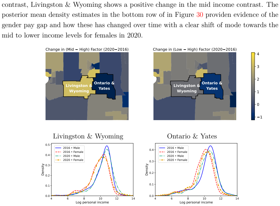
These PUMAs are Livingston & Wyoming and Ontario & Yates the heatmaps fo which are displayed in the top row with the corresponding posterior mean densities of log personal income for males and females displayed in bottom row. Ontario & Yates exhibits negative changes in both the mid and low income contrasts from 2016 to 2020, indicating that over time the...
work page 2016
-
[54]
2 1 0 1 2 3 (a) Education-related effects Change in (Mid High) Factor (2020
work page 2020
-
[56]
3 2 1 0 1 2 (b) Race-related effects Change in (Mid High) Factor (2020
work page 2020
-
[57]
Change in (Low High) Factor (2020
work page 2020
-
[58]
1 0 1 2 3 4 (c) Gender-related effects Figure 27: New York: Heat maps of contrast changes of PUMA specific covariate effects from 2016 to 2020 for mid and low income factors. Baseline - high income factor, larger positive change (bright yellow) and larger negative change (dark blue). 46 Onondaga (Central) Livingston & Wyoming Tompkins Change in (Mid High)...
work page 2016
-
[59]
Onondaga (Central) Livingston & Wyoming Tompkins Change in (Low High) Factor (2020
work page 2020
-
[60]
2 1 0 1 2 3 Livingston & Wyoming Onondaga (Central) Tompkins 4 6 8 10 12 14 Log personal income 0.0 0.1 0.2 0.3 0.4 0.5Density 2016 BA+ 2016 Below BA 2020 BA+ 2020 Below BA 4 6 8 10 12 14 Log personal income 0.0 0.1 0.2 0.3 0.4 0.5Density 2016 BA+ 2016 Below BA 2020 BA+ 2020 Below BA 4 6 8 10 12 14 Log personal income 0.0 0.1 0.2 0.3 0.4Density 2016 BA+ 2...
work page 2016
-
[61]
Onondaga (Central) Fulton & Montgomery Otsego & Schoharie Change in (Low High) Factor (2020
work page 2020
-
[62]
Posterior mean densities of log personal income by Race (bottom row)
2 1 0 1 2 3 Onondago (Central) Otesgo & Schoharie Fulton & Montegomery 4 6 8 10 12 14 Log personal income 0.0 0.1 0.2 0.3 0.4Density 2016 White 2016 NonWhite 2020 White 2020 Non White 4 6 8 10 12 14 Log personal income 0.0 0.1 0.2 0.3 0.4Density 2016 White 2016 NonWhite 2020 White 2020 Non White 4 6 8 10 12 14 Log personal income 0.00 0.05 0.10 0.15 0.20 ...
work page 2016
-
[63]
Livingston & Wyoming Ontario & Yates Change in (Mid High) Factor (2020
work page 2020
-
[64]
Livingston & Wyoming Ontario & Yates Change in (Low High) Factor (2020
work page 2020
-
[65]
Posterior mean densities of log personal income by Gender (bottom row)
1 0 1 2 3 4 Livingston & Wyoming Ontario & Yates 4 6 8 10 12 14 Log personal income 0.0 0.1 0.2 0.3 0.4 0.5Density 2016 Male 2016 Female 2020 Male 2020 Female 4 6 8 10 12 14 Log personal income 0.0 0.1 0.2 0.3 0.4Density 2016 Male 2016 Female 2020 Male 2020 Female Figure 30: New York (zoom-in on Livingston & Wyoming, and Ontario & Yates): Changes in PUMA-...
work page 2016
-
[66]
The highlighted PUMA exhibits a negative change in the low income factor contrast from 2016 to 2020, indicating that the education effect became more strongly associated with the 49 Education-related effects Race-related effects Gender-related effects 0.4 0.2 0.0 0.2 0.4 Figure 31: Washington: Heat maps of contrast changes of PUMA specific covariate effec...
work page 2016
-
[67]
0.6 0.4 0.2 0.0 0.2 0.4 0.6 0.8 1.0 4 6 8 10 12 14 Log personal income 0.0 0.1 0.2 0.3 0.4Density 2016 BA+ 2016 Below BA 2020 BA+ 2020 Below BA Figure 32: Washington (zoom-in on Seattle Northwest): Changes in PUMA-specific effects of Education (high income factor as baseline) from 2016 to 2020 (top row). Posterior mean densities of log personal income by ...
work page 2016
-
[68]
Posterior mean densities of log personal income by Education (bottom row)
0.4 0.2 0.0 0.2 0.4 0.6 4 6 8 10 12 14 Log personal income 0.00 0.05 0.10 0.15 0.20 0.25 0.30 0.35 0.40Density 2016 White 2016 NonWhite 2020 White 2020 Non White Figure 33: Washington (zoom-in on Bremerton & Port Orchard): Changes in PUMA-specific effects of Race (high income factor as baseline) from 2016 to 2020 (top row). Posterior mean densities of log...
work page 2016
-
[69]
The highlighted PUMA appears to show a negative change in the low factor contrast from 2016 to 2020, indicating that the race effect became less associated with the low-income factor over time. The posterior mean density estimates provide complementary evidence on how the income distributions of the White and Non-White populations evolved between 2016 and
work page 2016
discussion (0)
Sign in with ORCID, Apple, or X to comment. Anyone can read and Pith papers without signing in.