Bayesian integration G-formula for platform SMART designs allowing for adding new treatments
Pith reviewed 2026-05-07 15:39 UTC · model grok-4.3
The pith
Bayesian integration G-formula estimators allow valid comparison of treatment sequences in platform SMARTs that add new treatments over time.
A machine-rendered reading of the paper's core claim, the machinery that carries it, and where it could break.
Core claim
The central claim is that the BIG estimators, by using Bayesian models to integrate data across enrollment periods while respecting the platform design rules, produce consistent estimates of the effects of dynamic treatment regimes even when some treatment comparisons involve non-concurrent data.
What carries the argument
The Bayesian integration G-formula (BIG) estimators, which adapt the G-computation formula by placing a Bayesian model over period-specific parameters to pool information from concurrent and non-concurrent periods under the platform assumptions.
If this is right
- BIG estimators can be applied directly to ongoing platform SMARTs to evaluate full sequences of treatments without discarding non-concurrent data.
- Simulations show the BIG estimators achieve lower bias and better coverage than methods that ignore the platform structure.
- The method is demonstrated on the SNAP trial, illustrating how it produces estimates for treatment sequences involving newly added arms.
- The approach supports master-protocol designs in which the set of available treatments changes while patient outcomes continue to be observed.
Where Pith is reading between the lines
- If the integration works as claimed, the same Bayesian pooling idea could be tested in platform trials that are not SMARTs, such as those with continuous biomarker-guided adaptation.
- A direct extension would be to examine how sensitive the estimates are to different choices of prior distributions on the period-specific parameters.
- The framework raises the question of how to update recommended dynamic treatment regimes in real time as new arms are added and more non-concurrent data accumulate.
Load-bearing premise
The Bayesian model is correctly specified for how data integrate across periods and that non-concurrent observations can be validly combined without bias under the platform design.
What would settle it
Run a simulation of a platform SMART in which the true dynamic treatment regime effects are known and the Bayesian model is deliberately misspecified; if the BIG point estimates and intervals deviate systematically from the known values while a concurrent-only analysis does not, the claim is falsified.
Figures


read the original abstract
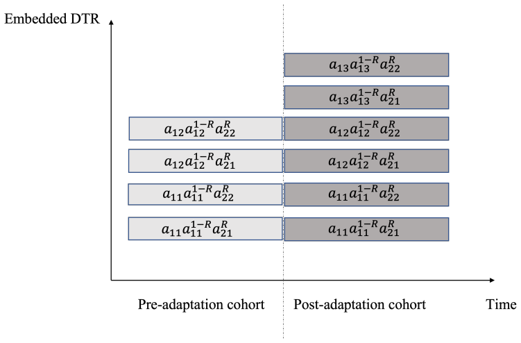
Dynamic treatment regimes (DTRs) are sequences of decision rules to guide treatment assignments in response to a patient's evolving, time-varying disease status. Sequential multiple assignment randomized trials (SMARTs) are considered the gold standard experimental design for evaluating DTRs. However, SMARTs often require more time to complete compared with a single stage RCT and new candidate treatments may become available or feasible during the trial. Platform trials are an adaptive trial design that allow new treatments to be added to the ongoing study according to a prespecified master protocol. In this paper, we introduce a novel platform SMART that integrates features from both platform trials and SMARTs, allowing new treatments to be added during the trial. Additionally, we propose the Bayesian integration G-formula (BIG) estimators for platform SMARTs to account for non-concurrent treatment comparisons. Extensive simulations are conducted to evaluate the performance of different BIG estimators against benchmark methods. We demonstrate the proposed BIG estimators based on the S. aureus Network Adaptive Platform (SNAP) trial.
Editorial analysis
A structured set of objections, weighed in public.
Referee Report
Summary. The manuscript introduces platform SMART designs, which extend standard SMARTs by allowing new treatments to be added during the trial according to a master protocol. It proposes Bayesian integration G-formula (BIG) estimators that integrate concurrent and non-concurrent data to estimate dynamic treatment regime values while accounting for potential differences across periods. The approach is evaluated through simulations comparing BIG variants to benchmark methods and is illustrated using data from the S. aureus Network Adaptive Platform (SNAP) trial.
Significance. If the BIG estimators are shown to be valid and robust, the work would enable more efficient and timely evaluation of DTRs in adaptive platform settings by permitting principled borrowing of non-concurrent information. The provision of simulation benchmarks and a real-trial application (SNAP) strengthens the practical contribution, though the central claim hinges on the untested integration assumptions.
major comments (2)
- [Simulation Study] Simulation Study section: The manuscript states that extensive simulations evaluate the performance of the BIG estimators, but provides no explicit description of the data-generating mechanisms, including how period-specific effects, time trends, or eligibility changes are simulated. Without these details, it is impossible to assess whether the reported bias, coverage, and efficiency gains hold under realistic violations of the no-unmodeled-time-trends assumption.
- [Methods] Methods section on BIG estimators: The validity of non-concurrent borrowing rests on the Bayesian model correctly specifying the integration kernel across periods (stable eligibility, no unmodeled population shifts). The paper does not include sensitivity analyses or alternative specifications (e.g., time-varying intercepts or misspecified priors) to quantify how bias in DTR value estimates propagates when these assumptions are violated.
minor comments (2)
- [Abstract] The abstract would benefit from a one-sentence statement of the key modeling assumptions required for the BIG estimators to be consistent.
- [Methods] Notation for the platform G-formula and the integration prior could be clarified with a small numerical example in the Methods section.
Simulated Author's Rebuttal
Thank you for the constructive feedback on our manuscript. We address each of the major comments point by point below and will revise the manuscript to incorporate the suggested improvements.
read point-by-point responses
-
Referee: [Simulation Study] Simulation Study section: The manuscript states that extensive simulations evaluate the performance of the BIG estimators, but provides no explicit description of the data-generating mechanisms, including how period-specific effects, time trends, or eligibility changes are simulated. Without these details, it is impossible to assess whether the reported bias, coverage, and efficiency gains hold under realistic violations of the no-unmodeled-time-trends assumption.
Authors: We agree that the data-generating mechanisms require more explicit description to allow readers to evaluate the simulation results under the stated assumptions. In the revised manuscript, we will add a dedicated subsection in the Simulation Study that details the full data-generating process, including the models and parameters for period-specific effects, time trends, and eligibility changes. revision: yes
-
Referee: [Methods] Methods section on BIG estimators: The validity of non-concurrent borrowing rests on the Bayesian model correctly specifying the integration kernel across periods (stable eligibility, no unmodeled population shifts). The paper does not include sensitivity analyses or alternative specifications (e.g., time-varying intercepts or misspecified priors) to quantify how bias in DTR value estimates propagates when these assumptions are violated.
Authors: We concur that sensitivity analyses are essential to demonstrate robustness when integration assumptions are violated. In the revision, we will incorporate additional simulation scenarios that introduce violations such as unmodeled time trends, population shifts, and alternative prior specifications, reporting the resulting effects on bias, coverage, and efficiency of the DTR value estimates. revision: yes
Circularity Check
No significant circularity; BIG estimators derive independently from G-formula and Bayesian principles with external simulation validation
full rationale
The paper's derivation introduces Bayesian integration G-formula estimators by adapting the standard G-formula to platform SMART structures for non-concurrent comparisons. This relies on explicit modeling assumptions for period integration and borrowing, not on redefining the target estimand in terms of itself. Simulations evaluate performance against separate benchmark methods rather than fitting parameters to the outcome being predicted. No load-bearing self-citations, uniqueness theorems from prior author work, or smuggled ansatzes appear in the core estimator construction. The chain remains self-contained against external benchmarks.
Axiom & Free-Parameter Ledger
Reference graph
Works this paper leans on
-
[1]
Berry, S. M., Connor, J. T., and Lewis, R. J. (2015). The platform trial: an efficient strategy for evaluating multiple treatments.JAMA, 313(16):1619–1620. Bofill Roig, M., Burgwinkel, C., Garczarek, U., Koenig, F., Posch, M., Nguyen, Q., and Hees, K. (2023). On the use of non-concurrent controls in platform trials: a scoping review.Trials, 24(1):1–17. Ch...
work page 2015
-
[2]
Hobbs, B. P., Sargent, D. J., and Carlin, B. P. (2012). Commensurate priors for incorporating historical infor- mation in clinical trials using general and generalized linear models.Bayesian Analysis (Online), 7(3):639. Keil, A. P., Daza, E. J., Engel, S. M., Buckley, J. P., and Edwards, J. K. (2018). A bayesian approach to the g-formula.Statistical Metho...
work page 2012
-
[3]
Ko, J. H. and Wahed, A. S. (2012). Up-front versus sequential randomizations for inference on adaptive treatment strategies.Statistics in Medicine, 31(9):812–830. Krotka, P., Hees, K., Jacko, P., Magirr, D., Posch, M., and Roig, M. B. (2023). Ncc: An r-package for analysis and simulation of platform trials with non-concurrent controls.SoftwareX, 23:101437...
work page 2012
-
[4]
Wang, X. and Chakraborty, B. (2023). The sequential multiple assignment randomized trial for controlling infectious diseases: A review of recent developments.American Journal of Public Health, 113(1):49–59. Wi´ sniowski, A., Sakshaug, J. W., Perez Ruiz, D. A., and Blom, A. G. (2020). Integrating probability and nonprobability samples for survey inference....
work page 2023
-
[5]
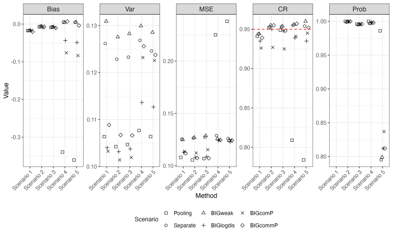
‘Prob’ represents the probability of identifying the true optimal DTR. BIGweak, BIGlogdis, BIGcomP and BIGcommP are the Bayesian integration g-formula (BIG) approaches with weakly informative priors, log distance priors, commensurate priors, and mixed commensurate priors. B Application results Figure 13: Application results withn= 2000 andr= 0.3. ‘Bias’, ...
work page 2000
-
[6]
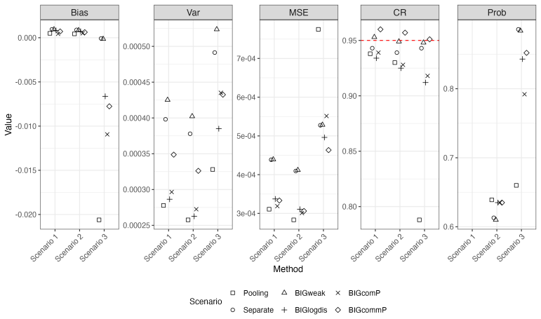
‘Prob’ represents the probability of identifying the true optimal DTR. BIGweak, BIGlogdis, BIGcomP and BIGcommP are the Bayesian integration g-formula (BIG) approaches with weakly informative priors, log distance priors, commensurate priors, and mixed commensurate priors. 21 Figure 14: Application results withn= 2000 andr= 0.7. ‘Bias’, ‘Var’, ‘MSE’, and ‘...
work page 2000
discussion (0)
Sign in with ORCID, Apple, or X to comment. Anyone can read and Pith papers without signing in.