Beyond Independence: on Jointly Normal Priors in Bayesian Inversion
Pith reviewed 2026-05-09 19:47 UTC · model grok-4.3
The pith
Jointly normal priors can include correlations between parameters while exactly preserving each parameter's marginal distribution.
A machine-rendered reading of the paper's core claim, the machinery that carries it, and where it could break.
Core claim
We construct jointly Gaussian prior models with prescribed Gaussian marginals so that correlation between the parameters can be incorporated without altering the marginal prior distributions. We propose a joint covariance construction that preserves the marginals, allows spatially varying cross-correlation, and supports uncertainty and inference in the correlation itself. The construction is valid for any strict contraction encoding the desired cross-correlation and is optimal in a canonical correlation sense under the principal square root factorisation. Demonstrations via prior sampling and inference examples, including a PDE-constrained problem, highlight pitfalls of ignoring correlation,
What carries the argument
The joint covariance construction that uses strict contraction factors to encode cross-correlations while preserving the given marginal distributions.
If this is right
- Spatially varying cross-correlations can be included without changing the marginal prior distributions.
- The strength of the correlation can be treated as a random variable and inferred jointly with the parameters.
- The construction remains valid for any strict contraction that encodes the desired cross-correlation.
- Neglecting uncertainty in the correlation produces incorrect posterior uncertainty estimates in the examples.
Where Pith is reading between the lines
- Routine inclusion of correlation as an inferred quantity would reduce bias in uncertainty estimates for many joint inversion tasks.
- The optimality property under principal square root factorization could guide choices among different matrix factorizations in similar constructions.
Load-bearing premise
The desired cross-correlations between parameters can always be represented by a strict contraction factor without producing invalid non-positive-definite joint covariances or violating the prescribed marginal distributions.
What would settle it
A concrete calculation for some choice of marginal variances and contraction factor that yields a joint covariance matrix with a negative eigenvalue would disprove the claim that the construction is always valid.
Figures


read the original abstract
We consider joint inversion for two or more unknown parameters from observational data in the Bayesian framework. Standard approaches often either treat the parameters as independent or impose structural similarity through regularisation terms that can be difficult to interpret statistically. We instead construct jointly Gaussian prior models with prescribed Gaussian marginals, so that correlation between the parameters can be incorporated without altering the marginal prior distributions. We propose a joint covariance construction that preserves the marginals, allows spatially varying cross-correlation, and supports uncertainty and inference in the correlation itself. The construction is valid for any strict contraction encoding the desired cross-correlation and is optimal in a canonical correlation sense under the principal square root factorisation. We demonstrate the method using prior sampling and several inference examples: a low-dimensional illustrative example and two higher-dimensional examples, including a PDE-constrained problem. The examples highlight both the potential pitfalls of ignoring or neglecting uncertainty in the correlation as well as reinforcing a key principle of the Bayesian paradigm: unknown quantities included in a model should be treated as random variables.
Editorial analysis
A structured set of objections, weighed in public.
Referee Report
Summary. The paper proposes a construction for jointly Gaussian prior models in Bayesian inversion of multiple parameters. It preserves prescribed Gaussian marginal distributions while incorporating cross-correlations via any strict contraction factor, with the joint covariance claimed to be valid for any such contraction and optimal in a canonical correlation sense under the principal square root factorization. The approach is illustrated through prior sampling and inference examples, including a low-dimensional case, higher-dimensional cases, and a PDE-constrained problem, with emphasis on treating correlation uncertainty as random.
Significance. If the central construction holds, the work offers a statistically grounded alternative to independence assumptions or ad-hoc regularization in multi-parameter Bayesian inversions. It enables spatially varying correlations without distorting marginal priors and supports inference on the correlation structure itself. The examples demonstrate practical value in uncertainty quantification, particularly for PDE-constrained settings, and align with core Bayesian principles by randomizing unknown quantities like correlations.
major comments (2)
- [Construction and theoretical claims (likely §3 or equivalent)] The abstract and introduction assert validity for any strict contraction and optimality under principal square root factorization, but the manuscript does not provide the explicit matrix construction or step-by-step verification that the resulting joint covariance remains positive definite while exactly preserving the marginal covariances. This verification is load-bearing for the central claim; without it, the support for the proposal cannot be fully assessed from the given examples alone.
- [Examples and PDE-constrained demonstration] The weakest assumption—that any desired cross-correlation can be encoded by a strict contraction without producing non-positive-definite joints—is stated but not accompanied by a general proof or counterexample analysis. The low-dimensional example may satisfy it by construction, but this needs explicit confirmation for the higher-dimensional and PDE cases to substantiate the broad applicability.
minor comments (2)
- [Notation and setup] Notation for the contraction factor and factorization could be introduced with a dedicated table or diagram early in the paper to improve readability for readers unfamiliar with canonical correlation analysis.
- [Numerical results] The discussion of pitfalls when ignoring correlation uncertainty would be strengthened by a direct quantitative comparison (e.g., posterior variance or credible interval width) between the proposed joint model and an independence baseline in one of the numerical examples.
Simulated Author's Rebuttal
We thank the referee for the constructive and detailed report, which highlights both the potential value of the proposed joint prior construction and areas where the presentation can be strengthened. We address each major comment below and will incorporate the requested clarifications and verifications into the revised manuscript.
read point-by-point responses
-
Referee: [Construction and theoretical claims (likely §3 or equivalent)] The abstract and introduction assert validity for any strict contraction and optimality under principal square root factorization, but the manuscript does not provide the explicit matrix construction or step-by-step verification that the resulting joint covariance remains positive definite while exactly preserving the marginal covariances. This verification is load-bearing for the central claim; without it, the support for the proposal cannot be fully assessed from the given examples alone.
Authors: We agree that the central claim requires explicit support. The manuscript defines the joint covariance via the principal square-root factorization of the marginal covariances combined with a contraction operator, but we acknowledge that a self-contained derivation of positive definiteness and exact marginal preservation is not fully expanded. In the revision we will add, in the theoretical section, the explicit block-matrix expression together with a short proof: the Schur complement of the joint matrix reduces to a positive-definite term precisely when the contraction has spectral radius strictly less than one, while the diagonal blocks recover the prescribed marginal covariances by construction. This will be accompanied by the canonical-correlation optimality argument under the principal-square-root choice. revision: yes
-
Referee: [Examples and PDE-constrained demonstration] The weakest assumption—that any desired cross-correlation can be encoded by a strict contraction without producing non-positive-definite joints—is stated but not accompanied by a general proof or counterexample analysis. The low-dimensional example may satisfy it by construction, but this needs explicit confirmation for the higher-dimensional and PDE cases to substantiate the broad applicability.
Authors: We accept that a general statement without supporting analysis is insufficient. The low-dimensional example is verified directly, but the higher-dimensional and PDE examples rely on the same contraction mechanism without separate confirmation. In the revision we will insert a concise general lemma establishing that any strict contraction (operator norm <1) yields a positive-definite joint while leaving marginals unchanged, together with a short remark on the boundary case of non-strict contractions. We will also add a brief numerical check of the smallest eigenvalue of the joint covariance in the two higher-dimensional examples (including the PDE-constrained case) to illustrate that the property holds in practice. revision: yes
Circularity Check
No significant circularity
full rationale
The paper presents a direct mathematical construction for jointly Gaussian priors that preserves prescribed marginals via any strict contraction factor and principal square root factorization. This is an explicit definition of the joint covariance (valid by the contraction property and optimality under canonical correlation), not a reduction of a target quantity to fitted inputs, self-referential equations, or load-bearing self-citations. The examples illustrate the construction without deriving the core result from the data or prior outputs. The derivation chain is self-contained as a proposal of a new prior model.
Axiom & Free-Parameter Ledger
free parameters (1)
- contraction factor
axioms (2)
- domain assumption Parameters follow jointly Gaussian distributions with prescribed Gaussian marginals
- domain assumption A strict contraction can represent any desired cross-correlation structure
Reference graph
Works this paper leans on
-
[1]
Joint two-dimensional DC resistivity and seismic travel time inversion with cross-gradients constraints.Journal of Geophysical Research: Solid Earth, 109(B3), 2004
Luis A Gallardo and Max A Meju. Joint two-dimensional DC resistivity and seismic travel time inversion with cross-gradients constraints.Journal of Geophysical Research: Solid Earth, 109(B3), 2004
2004
-
[2]
Joint inversion approaches for geophysical electromagnetic and elastic full-waveform data.Inverse Problems, 28(5):055016, 2012
Aria Abubakar, G Gao, Tarek M Habashy, and J Liu. Joint inversion approaches for geophysical electromagnetic and elastic full-waveform data.Inverse Problems, 28(5):055016, 2012
2012
-
[3]
Estimation of field-scale soil hydraulic and dielectric parameters through joint inversion of GPR and hydrological data.Water Resources Research, 41(11), 2005
Michael B Kowalsky, Stefan Finsterle, John Peterson, Susan Hubbard, Yoram Rubin, Ernest Majer, Andy Ward, and Glendon Gee. Estimation of field-scale soil hydraulic and dielectric parameters through joint inversion of GPR and hydrological data.Water Resources Research, 41(11), 2005
2005
-
[4]
Model fusion and joint inversion.Surveys in Geophysics, 34(5):675– 695, 2013
Eldad Haber and Michal Holtzman Gazit. Model fusion and joint inversion.Surveys in Geophysics, 34(5):675– 695, 2013
2013
-
[5]
Study on joint inversion algorithm of acoustic and electromagnetic data in biomedical imaging.IEEE Journal on Multiscale and Multiphysics Computational Techniques, 4:2–11, 2019
Xiaoqian Song, Maokun Li, Fan Yang, Shenheng Xu, and Aria Abubakar. Study on joint inversion algorithm of acoustic and electromagnetic data in biomedical imaging.IEEE Journal on Multiscale and Multiphysics Computational Techniques, 4:2–11, 2019
2019
-
[6]
Joint reconstruction of PET-MRI by exploiting structural similarity.Inverse Problems, 31(1):015001, 2014
Matthias J Ehrhardt, Kris Thielemans, Luis Pizarro, David Atkinson, S´ ebastien Ourselin, Brian F Hutton, and Simon R Arridge. Joint reconstruction of PET-MRI by exploiting structural similarity.Inverse Problems, 31(1):015001, 2014
2014
-
[7]
Joint reconstruction via coupled Bregman iterations 23 with applications to PET-MR imaging.Inverse Problems, 34(1):014001, 2017
Julian Rasch, Eva-Maria Brinkmann, and Martin Burger. Joint reconstruction via coupled Bregman iterations 23 with applications to PET-MR imaging.Inverse Problems, 34(1):014001, 2017
2017
-
[8]
Corrosion detection in conducting boundaries.Inverse Problems, 20(4):1207, 2004
G Inglese and F Mariani. Corrosion detection in conducting boundaries.Inverse Problems, 20(4):1207, 2004
2004
-
[9]
Ruanui Nicholson and Matti Niskanen. Joint estimation of Robin coefficient and domain boundary for the Poisson problem.arXiv preprint arXiv:2108.09152, 2021
-
[10]
Springer Science & Business Media, 2003
Hans Wackernagel.Multivariate geostatistics: an introduction with applications. Springer Science & Business Media, 2003
2003
-
[11]
John Wiley & Sons, 2012
Jean-Paul Chiles and Pierre Delfiner.Geostatistics: modeling spatial uncertainty. John Wiley & Sons, 2012
2012
-
[12]
A comparative study of regularizations for joint inverse problems.Inverse Problems, 35(2), 2018
Benjamin Crestel, Georg Stadler, and Omar Ghattas. A comparative study of regularizations for joint inverse problems.Inverse Problems, 35(2), 2018
2018
-
[13]
Can one use total variation prior for edge-preserving Bayesian inversion? Inverse Problems, 20(5):1537, 2004
Matti Lassas and Samuli Siltanen. Can one use total variation prior for edge-preserving Bayesian inversion? Inverse Problems, 20(5):1537, 2004
2004
-
[14]
A framework for time-dependent ice sheet uncertainty quantification, applied to three west antarctic ice streams.The Cryosphere, 17(10):4241–4266, 2023
Beatriz Recinos, Daniel Goldberg, James R Maddison, and Joe Todd. A framework for time-dependent ice sheet uncertainty quantification, applied to three west antarctic ice streams.The Cryosphere, 17(10):4241–4266, 2023
2023
-
[15]
An inexact gauss-newton method for inversion of basal sliding and rheology parameters in a nonlinear stokes ice sheet model.Journal of Glaciology, 58(211):889–903, 2012
Noemi Petra, Hongyu Zhu, Georg Stadler, Thomas JR Hughes, and Omar Ghattas. An inexact gauss-newton method for inversion of basal sliding and rheology parameters in a nonlinear stokes ice sheet model.Journal of Glaciology, 58(211):889–903, 2012
2012
-
[16]
Niko H¨ anninen, Aki Pulkkinen, Aleksi Leino, and Tanja Tarvainen. Application of diffusion approximation in quantitative photoacoustic tomography in the presence of low-scattering regions.Journal of Quantitative Spectroscopy and Radiative Transfer, 250:107065, 2020
2020
-
[17]
Computing the nearest correlation matrix—a problem from finance.IMA journal of Numerical Analysis, 22(3):329–343, 2002
Nicholas J Higham. Computing the nearest correlation matrix—a problem from finance.IMA journal of Numerical Analysis, 22(3):329–343, 2002
2002
-
[18]
Least-squares covariance matrix adjustment.SIAM Journal on Matrix Analysis and Applications, 27(2):532–546, 2005
Stephen Boyd and Lin Xiao. Least-squares covariance matrix adjustment.SIAM Journal on Matrix Analysis and Applications, 27(2):532–546, 2005
2005
-
[19]
A quadratically convergent Newton method for computing the nearest correlation matrix.SIAM journal on matrix analysis and applications, 28(2):360–385, 2006
Houduo Qi and Defeng Sun. A quadratically convergent Newton method for computing the nearest correlation matrix.SIAM journal on matrix analysis and applications, 28(2):360–385, 2006
2006
-
[20]
An application of the nearest correlation matrix on web document classification.Journal of Industrial and Management Optimization, 3(4):701, 2007
Houduo Qi, Zhonghang Xia, and Guangming Xing. An application of the nearest correlation matrix on web document classification.Journal of Industrial and Management Optimization, 3(4):701, 2007
2007
-
[21]
Computing a nearest correlation matrix with factor structure.SIAM Journal on Matrix Analysis and Applications, 31(5):2603–2622, 2010
R¨ udiger Borsdorf, Nicholas J Higham, and Marcos Raydan. Computing a nearest correlation matrix with factor structure.SIAM Journal on Matrix Analysis and Applications, 31(5):2603–2622, 2010
2010
-
[22]
Bounds for the distance to the nearest correlation matrix.SIAM Journal on Matrix Analysis and Applications, 37(3):1088–1102, 2016
Nicholas J Higham and Natasa Strabic. Bounds for the distance to the nearest correlation matrix.SIAM Journal on Matrix Analysis and Applications, 37(3):1088–1102, 2016
2016
-
[23]
Inverse problems: A Bayesian perspective.Acta Numerica, 19:451–559, 2010
Andrew M Stuart. Inverse problems: A Bayesian perspective.Acta Numerica, 19:451–559, 2010
2010
-
[24]
Tan Bui-Thanh, Omar Ghattas, James Martin, and Georg Stadler. A computational framework for infinite- dimensional Bayesian inverse problems part I: The linearized case, with application to global seismic inver- sion.SIAM Journal on Scientific Computing, 35(6):A2494–A2523, 2013
2013
-
[25]
Noemi Petra, James Martin, Georg Stadler, and Omar Ghattas. A computational framework for infinite- dimensional Bayesian inverse problems, part II: Stochastic Newton MCMC with application to ice sheet flow inverse problems.SIAM Journal on Scientific Computing, 36(4):A1525–A1555, 2014
2014
-
[26]
Springer-Verlag New York, 2005
Jari Kaipio and Erkki Somersalo.Statistical and Computational Inverse Problems, volume 160 ofApplied Mathematical Sciences. Springer-Verlag New York, 2005
2005
-
[27]
Springer Science & Business Media, 2007
Daniela Calvetti and Erkki Somersalo.An introduction to Bayesian scientific computing: ten lectures on subjective computing, volume 2. Springer Science & Business Media, 2007
2007
-
[28]
Kaipio and V
J.P. Kaipio and V. Kolehmainen.Approximate Marginalization Over Modeling Errors and Uncertainties in Inverse Problems, chapter 32, pages 644–672. Oxford University Press, 2013
2013
-
[29]
Iterative updating of model error for Bayesian inversion.Inverse Problems, 34(2):025008, 2018
Daniela Calvetti, Matthew Dunlop, Erkki Somersalo, and Andrew M Stuart. Iterative updating of model error for Bayesian inversion.Inverse Problems, 34(2):025008, 2018
2018
-
[30]
Estimation of the Robin coefficient field in a Poisson problem with uncertain conductivity field.Inverse Problems, 34(11):115005, 2018
Ruanui Nicholson, Noemi Petra, and Jari P Kaipio. Estimation of the Robin coefficient field in a Poisson problem with uncertain conductivity field.Inverse Problems, 34(11):115005, 2018
2018
-
[31]
Inferring the basal sliding coefficient field for the Stokes ice sheet model under rheological uncertainty.The Cryosphere, 15(4):1731–1750, 2021
Olalekan Babaniyi, Ruanui Nicholson, Umberto Villa, and Noemi Petra. Inferring the basal sliding coefficient field for the Stokes ice sheet model under rheological uncertainty.The Cryosphere, 15(4):1731–1750, 2021
2021
-
[32]
Whittle-Mat´ ern priors for Bayesian statistical inversion with applications in electrical impedance tomography.Inverse Problems & Imaging, 8(2):561, 2014
Lassi Roininen, Janne MJ Huttunen, and Sari Lasanen. Whittle-Mat´ ern priors for Bayesian statistical inversion with applications in electrical impedance tomography.Inverse Problems & Imaging, 8(2):561, 2014
2014
-
[33]
Inverse problems with structural prior information.Inverse problems, 15(3):713, 1999
Jari P Kaipio, Ville Kolehmainen, Marko Vauhkonen, and Erkki Somersalo. Inverse problems with structural prior information.Inverse problems, 15(3):713, 1999
1999
-
[34]
Inverse problems: From regularization to Bayesian inference.Wiley Interdisciplinary Reviews: Computational Statistics, 10(3):e1427, 2018
Daniela Calvetti and Erkki Somersalo. Inverse problems: From regularization to Bayesian inference.Wiley Interdisciplinary Reviews: Computational Statistics, 10(3):e1427, 2018
2018
-
[35]
Finn Lindgren, H˚ avard Rue, and Johan Lindstr¨ om. An explicit link between Gaussian fields and Gaussian Markov random fields: The stochastic partial differential equation approach.Journal of the Royal Statistical Society: Series B (Statistical Methodology), 73(4):423–498, 2011
2011
-
[36]
Cauchy Markov random field priors for Bayesian inversion
Neil K Chada, Lassi Roininen, and Jarkko Suuronen. Cauchy Markov random field priors for Bayesian inversion. arXiv preprint arXiv:2105.12488, 2021
-
[37]
Gaussian cosimulation: Modelling of the cross-covariance.Mathematical Geology, 35(6):681–698, 24 2003
Dean S Oliver. Gaussian cosimulation: Modelling of the cross-covariance.Mathematical Geology, 35(6):681–698, 24 2003
2003
-
[38]
Cambridge university press, 2012
Roger A Horn and Charles R Johnson.Matrix analysis. Cambridge university press, 2012
2012
-
[39]
John Wiley & Sons, Ltd, 2003
Theodore Wilbur Anderson.An Introduction to Multivariate Statistical Analysis, volume 3. John Wiley & Sons, Ltd, 2003
2003
-
[40]
Relations between two sets of variates.Biometrika, 28(3-4):321–377, 1936
Harold Hotelling. Relations between two sets of variates.Biometrika, 28(3-4):321–377, 1936
1936
-
[41]
Mitigating the influence of the boundary on PDE-based covariance operators
Yair Daon and Georg Stadler. Mitigating the influence of the boundary on PDE-based covariance operators. Inverse Problems & Imaging, 12(5):1083, 2018
2018
-
[42]
Analysis of boundary effects on PDE-based sampling of Whittle–Mat´ ern random fields.SIAM/ASA Journal on Uncertainty Quantification, 7(3):948–974, 2019
Ustim Khristenko, Laura Scarabosio, Piotr Swierczynski, Elisabeth Ullmann, and Barbara Wohlmuth. Analysis of boundary effects on PDE-based sampling of Whittle–Mat´ ern random fields.SIAM/ASA Journal on Uncertainty Quantification, 7(3):948–974, 2019
2019
-
[43]
Carl Edward Rasmussen and Christopher K. I. Williams.Gaussian Processes for Machine Learning. MIT Press, 2005
2005
-
[44]
JHU press, 2013
Gene H Golub and Charles F Van Loan.Matrix computations. JHU press, 2013
2013
-
[45]
Hierarchical bayesian level set inversion.Statistics and Computing, 27(6):1555–1584, 2017
Matthew M Dunlop, Marco A Iglesias, and Andrew M Stuart. Hierarchical bayesian level set inversion.Statistics and Computing, 27(6):1555–1584, 2017
2017
-
[46]
Springer, 1999
Christian P Robert, George Casella, and George Casella.Monte Carlo statistical methods, volume 2. Springer, 1999
1999
-
[47]
Analysis of the gibbs sampler for hierarchical inverse problems.SIAM/ASA Journal on Uncertainty Quantification, 2(1):511–544, 2014
Sergios Agapiou, Johnathan M Bardsley, Omiros Papaspiliopoulos, and Andrew M Stuart. Analysis of the gibbs sampler for hierarchical inverse problems.SIAM/ASA Journal on Uncertainty Quantification, 2(1):511–544, 2014
2014
-
[48]
Hyperpriors for mat´ ern fields with applications in bayesian inversion.Inverse Problems & Imaging, 13(1), 2019
Lassi Roininen, Mark Girolami, Sari Lasanen, and Markku Markkanen. Hyperpriors for mat´ ern fields with applications in bayesian inversion.Inverse Problems & Imaging, 13(1), 2019
2019
-
[49]
A metropolis-hastings-within-gibbs sampler for nonlinear hierarchical-bayesian inverse problems
Johnathan M Bardsley and Tiangang Cui. A metropolis-hastings-within-gibbs sampler for nonlinear hierarchical-bayesian inverse problems. In2017 MATRIX Annals, pages 3–12. Springer, 2019
2019
-
[50]
Principal component analysis.Encyclopedia of statistics in behavioral science, 2005
Ian Jolliffe. Principal component analysis.Encyclopedia of statistics in behavioral science, 2005
2005
-
[51]
Electrical impedance tomography imaging with reduced- order model based on proper orthogonal decomposition.Journal of Electronic Imaging, 22(2):023008, 2013
Antti Lipponen, Aku Seppanen, and Jari P Kaipio. Electrical impedance tomography imaging with reduced- order model based on proper orthogonal decomposition.Journal of Electronic Imaging, 22(2):023008, 2013
2013
-
[52]
Survey of multifidelity methods in uncertainty propagation, inference, and optimization.Siam Review, 60(3):550–591, 2018
Benjamin Peherstorfer, Karen Willcox, and Max Gunzburger. Survey of multifidelity methods in uncertainty propagation, inference, and optimization.Siam Review, 60(3):550–591, 2018
2018
-
[53]
Chapman and Hall/CRC, 1995
Andrew Gelman, John B Carlin, Hal S Stern, and Donald B Rubin.Bayesian data analysis. Chapman and Hall/CRC, 1995
1995
-
[54]
Maximum a posteriori probability estimates in infinite-dimensional Bayesian inverse problems.Inverse Problems, 31(8):085009, 2015
Tapio Helin and Martin Burger. Maximum a posteriori probability estimates in infinite-dimensional Bayesian inverse problems.Inverse Problems, 31(8):085009, 2015
2015
-
[55]
MAP estimators and their consistency in Bayesian nonparametric inverse problems.Inverse Problems, 29(9):095017, 2013
Masoumeh Dashti, Kody JH Law, Andrew M Stuart, and Jochen Voss. MAP estimators and their consistency in Bayesian nonparametric inverse problems.Inverse Problems, 29(9):095017, 2013
2013
-
[56]
The monod model and its alternatives
Arthur L Koch. The monod model and its alternatives. InMathematical modeling in microbial ecology, pages 62–93. Springer, 1998
1998
-
[57]
Randomize-then-optimize: A method for sampling from posterior distributions in nonlinear inverse problems.SIAM Journal on Scientific Com- puting, 36(4):A1895–A1910, 2014
Johnathan M Bardsley, Antti Solonen, Heikki Haario, and Marko Laine. Randomize-then-optimize: A method for sampling from posterior distributions in nonlinear inverse problems.SIAM Journal on Scientific Com- puting, 36(4):A1895–A1910, 2014
2014
-
[58]
An adaptive Metropolis algorithm.Bernoulli, 7(2):223 – 242, 2001
Heikki Haario, Eero Saksman, and Johanna Tamminen. An adaptive Metropolis algorithm.Bernoulli, 7(2):223 – 242, 2001
2001
-
[59]
A tutorial on adaptive mcmc.Statistics and computing, 18:343–373, 2008
Christophe Andrieu and Johannes Thoms. A tutorial on adaptive mcmc.Statistics and computing, 18:343–373, 2008
2008
-
[60]
Weak convergence and optimal scaling of random walk metropolis algorithms.The annals of applied probability, 7(1):110–120, 1997
Andrew Gelman, Walter R Gilks, and Gareth O Roberts. Weak convergence and optimal scaling of random walk metropolis algorithms.The annals of applied probability, 7(1):110–120, 1997
1997
-
[61]
Hierarchical Bayesian models and sparsity:ℓ 2-magic.Inverse Problems, 35(3):035003, 2019
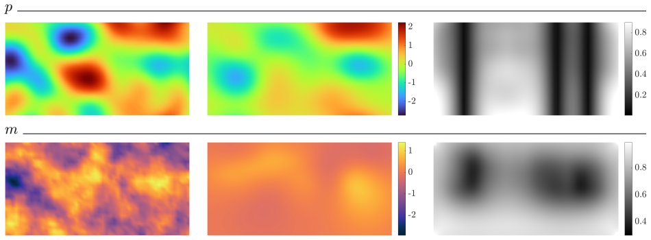
Daniela Calvetti, Erkki Somersalo, and A Strang. Hierarchical Bayesian models and sparsity:ℓ 2-magic.Inverse Problems, 35(3):035003, 2019. Appendix A. Illustration of the pitfall of optimisation when estimating the correlation. Here we provide some further insight into why optimisation-based approaches to estimating both parameterspandmas well as the corr...
2019
discussion (0)
Sign in with ORCID, Apple, or X to comment. Anyone can read and Pith papers without signing in.