pith. machine review for the scientific record. sign in

arxiv: 2605.03745 · v1 · submitted 2026-05-04 · ✦ hep-ex

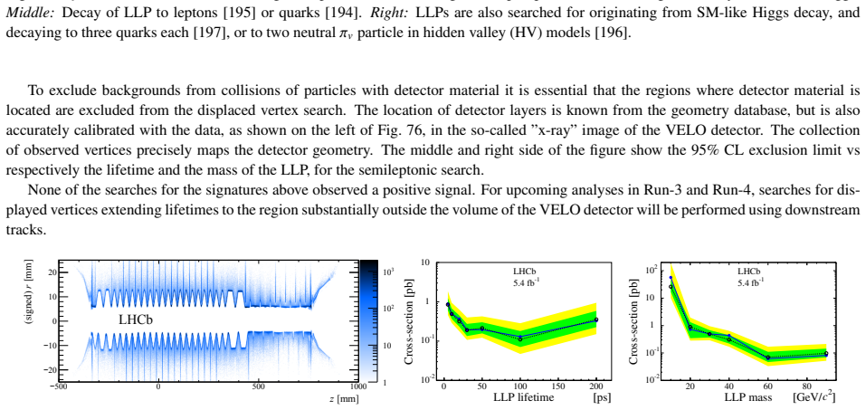
Recognition: unknown

The LHCb Experiment

Authors on Pith no claims yet

Pith reviewed 2026-05-08 02:29 UTC · model grok-4.3

classification ✦ hep-ex
keywords LHCbCP violationB mesonsforward spectrometerflavour physicsdetector upgraderare decaysheavy ions
0
0 comments X

The pith

LHCb started as a specialized B-meson experiment for CP violation but grew into a general-purpose forward spectrometer at the LHC while keeping its flavour-physics focus.

A machine-rendered reading of the paper's core claim, the machinery that carries it, and where it could break.

The paper traces how LHCb was built to measure CP violation and rare decays in B mesons at the LHC. It shows that the same forward geometry and detector choices later supported a much wider program including spectroscopy, long-lived particles, W and Z production, and heavy-ion studies. The review walks through the detector layout, the upgrade, and the analysis methods that turn raw hits into the observables used in those measurements. It ends with a comparison to other LHC experiments and a sketch of a second upgrade for the high-luminosity era.

Core claim

Originally conceived as a dedicated experiment for CP violation and rare decays in the B-meson sector, LHCb evolved into a general-purpose experiment for physics in the forward direction at the LHC, while maintaining its core optimization on flavour physics.

What carries the argument

The forward spectrometer geometry together with its vertex detector, tracking stations, and particle-identification systems that reconstruct events efficiently at small angles to the beam.

If this is right

  • LHCb delivers world-leading measurements of CP-violating phases and branching fractions in B decays.
  • The same apparatus supports searches for long-lived particles and spectroscopy of exotic hadrons.
  • Forward W and Z production data test electroweak theory at low Bjorken-x.
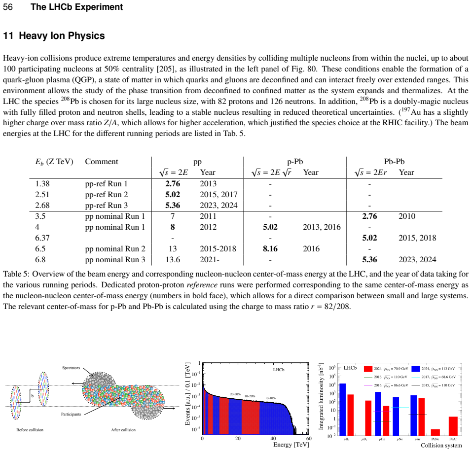
  • Heavy-ion runs yield nuclear modification factors in the forward region.
  • The first upgrade increases luminosity while preserving the core flavour-physics precision.

Where Pith is reading between the lines

These are editorial extensions of the paper, not claims the author makes directly.

  • A second upgrade at the HL-LHC would extend the same forward advantages to higher statistics and rarer processes.
  • The forward optimisation gives LHCb a distinct role compared with the central detectors at ATLAS and CMS in several channels.
  • The design choices that worked for B physics turn out to be broadly useful for any physics that produces particles at small angles.
  • Future data-taking periods could test whether the current analysis techniques remain efficient at the higher pile-up expected after the upgrade.

Load-bearing premise

The review assumes that the summarized detector components and analysis techniques accurately translate detailed detector information into reliable event-level observables for the listed physics topics.

What would settle it

Independent measurements from ATLAS or CMS that contradict the performance figures or physics results reported for the overlapping forward-rapidity region would undermine the claimed capabilities.

Figures

Figures reproduced from arXiv: 2605.03745 by Marcel H. M. Merk, Niels Tuning.

Figure 1
Figure 1. Figure 1: Display of an LHC event in the LHCb detector. The picture shows the layout of the forward spectrometer with a reconstructed view at source ↗
Figure 2
Figure 2. Figure 2: Schematic representations of the three precursor proposals: COBEX, GAJET and LHB. COBEX was designed as a collider mode view at source ↗
Figure 3
Figure 3. Figure 3: The evolution of the LHCb experiment from initial design to construction. The forward spectrometer evolved over time from the view at source ↗
Figure 4
Figure 4. Figure 4: The LHCb collaboration photoshopped into the experimental detector hall. CERN Document Server: CERN-PHOTO-202203-057. view at source ↗
Figure 5
Figure 5. Figure 5: Historically, the signs of the existence of many particles in the view at source ↗
Figure 6
Figure 6. Figure 6: Left: Layout of the LHCb spectrometer with from left to right the Vertex Locator, RICH-1, Upstream Tracker, Dipole Magnet, Downstream Tracker, RICH-1, Electromagnetic and Hadronic Calorimeters and Muon stations. Credit: CERN. Right: A schematic depic￾tion of the concepts of LHCb detector systems. Credit: Royal Society Summer Science Exhibition 2016. The LHCb-I experiment collected data during LHC Run-1 and… view at source ↗
Figure 7
Figure 7. Figure 7: Schematic views of Left: LHCb-I VELO radial (”R”) and azimuthal (”Phi”) sensor. Taken from [31]. Right: VELO LHCb-U pixel sensors on front and back side of modules. Taken from [36]. To accommodate the forward acceptance of LHCb, the Vertex Lo￾cator (VELO) is instrumented by a series of stations mounted per￾pendicular to the LHC beamline, close to the interaction region. The longitudinal size of the interac… view at source ↗
Figure 8
Figure 8. Figure 8: Schematic view of Longitudinal sensor positioning view at source ↗
Figure 9
Figure 9. Figure 9: The VELO half detector prior to installation. view at source ↗
Figure 10
Figure 10. Figure 10: Photographs of left: the LHCb Trigger Tracker [38] and right: the Upstream Tracker (CERN photograph), prior to their installation. For pattern recognition purposes the track￾ing station includes four measurement planes, la￾beled as x-u-v-x with respective stereo angles of 0, −5 o , +5 0 , 0 of the strips with respect to the ver￾tical y-axis. The detectors are mechanically con￾structed in two detector halv… view at source ↗
Figure 11
Figure 11. Figure 11: Schematic layout of four detector planes with stereo views view at source ↗
Figure 12
Figure 12. Figure 12: Left: Isometric view of the three Outer Tracker stations, where one side of the second station is displaced in the opened position. Center: Detection principles of the straw tube drift detector [41]. Right: View of the drift tube straws in inside an OT module [42]. The OT straw modules (see view at source ↗
Figure 13
Figure 13. Figure 13: Left: Isometric view of a single Inner Tracker detector station consisting of four detector boxes [31] Right: Photograph of the Si modules during their construction [43]. To accommodate the significantly increased track multiplicity in Run-3, LHCb-U replaced the OT straw tubes with a scintillating fiber tracker (SciFi), offering 20 times finer granularity. The SciFi detector layers consist of stacked scin… view at source ↗
Figure 14
Figure 14. Figure 14: Left: Detection principle of the fine-grained scintillating fibers read out by SiPMs [40]. The image schematically illustrates a track traversing the stack of fibers, the generated scintillation photons together with the response of the SiPM. Right: Photograph of SciFi detector plane prior to installation. The black surface represents the active detector region, the blue ends house the readout electronics… view at source ↗
Figure 15
Figure 15. Figure 15: Left: Schematic view of the LHCb dipole magnet. Center: Picture of the LHCb magnet after installation. The magnet coil is visible in yellow/lightbrown color and the yoke in red/brown. Right: Vertical (main) component of the B-field (By) along the beam axis (x = y = 0) for both polarities [31]. 3.3 Particle Identification Detectors Extensive particle identification (PID) is a key feature of the LHCb spectr… view at source ↗
Figure 16
Figure 16. Figure 16: The readout system is positioned outside the fiducial volume and used Hybrid Photon Detectors (HPDs) in LHCb-I, which could view at source ↗
Figure 16
Figure 16. Figure 16: Schematic view of the RICH detectors. Left: RICH-1, where particles enter at the left side via the VELO exit window. Emitted photons are reflected by the spherical mirror and a planar mirror onto photodetectors at the top and bottom. Right: RICH-2, where the spherical mirrors bring the photons to the photon detectors at the left and right side. Taken from [44] view at source ↗
Figure 17
Figure 17. Figure 17: Left: Photo of the spherical RICH-1 mirrors prior to installation (CERN Document Server). Right: Photo of the spherical RICH-2 mirrors with hexagon shapes on the right and the planar mirrors on the left. At the bottom center the photon detector system can be seen (CERN Document Server). 3.3.2 The Calorimeter System The calorimeter system provides identification for electrons, photons and hadrons as well a… view at source ↗
Figure 18
Figure 18. Figure 18: Photos of the calorimeter prior to installation. view at source ↗
Figure 19
Figure 19. Figure 19: Schematic view of an ECAL cell. Reproduced view at source ↗
Figure 20
Figure 20. Figure 20: Schematic view of an HCAL cell. Repro￾duced from [45]. The HCAL is a sampling calorimeter made from iron as absorber and active scintillating tiles, arranged in a structure running parallel to the beam axis (see view at source ↗
Figure 21
Figure 21. Figure 21: Left: Schematic view of the muon system comprising 5 muon stations M1 - M5 [31] Right: View from the floor of the cavern between the M1 and M2 muon detector planes. In the center of the picture the beampipe is seen (CERN Document Server). Muon identification is essential for both real-time triggering and offline analysis in flavour physics. The LHCb-I muon system consists of five stations (M1-M5), shown in view at source ↗
Figure 22
Figure 22. Figure 22: Real-time reconstruction and event selection scheme as used in LHCb-U, taken from LHCb-FIGURE-2020-016. view at source ↗
Figure 23
Figure 23. Figure 23: Left: Top view display of a reconstructed LHCb event, illustrating bending of the tracks in the dipole magnet field. Right: The different particle track-types, defined according to their acceptance in the experiment. Picture taken from [46]. A typical bb¯ event, shown on the left in Fig.23, consists of approximately 70 charged particle tracks when there is a single pp collision (i.e., no pile-up). These t… view at source ↗
Figure 25
Figure 25. Figure 25: The principle of the Kalman filter. Taken from [51]. view at source ↗
Figure 26
Figure 26. Figure 26: Left: Momentum resolution of the reconstructed muons from J/ψ particle decays expressed as δp/p vs momentum p, where δp is the estimated track error [57]. Right: Reconstructed di-muon mass spectrum where the Υ(1S ), Υ(2S ) and Υ(3S ) resonances are clearly distinguished and their mass resolutions are approximately 50 MeV [57] view at source ↗
Figure 27
Figure 27. Figure 27: Left: Sketch of the Bremsstrahlung recovery, by adding the energy of the radiated photon to the energy of the measured electron. Right: An event display from run 218585, 23 Nov 2018, illustrating the energy deposits in the ECAL and a photon being added to the electron e − . 4.1.4 Vertex reconstruction and decay time measurement The proton-proton collision point is referred to as the primary vertex (PV). T… view at source ↗
Figure 28
Figure 28. Figure 28: Left: The resolution of the impact parameter of the particle track to its production vertex as a function of the inverse transverse momentum 1/pT . The IPx is calculated as the distance in x between the extrapolated track and the vertex at the z = zvertex plane. Right: Precision of the reconstruction of the Primary Vertex as a function of the number of tracks, N, for projections in x-z plane (red) and y -… view at source ↗
Figure 29
Figure 29. Figure 29: Left: Schematic illustration of particle identification in LHCb [60]. Right: Charged particle identification performance using the RICH detectors [61]. To separate photons and merged π 0 particles, a multi-layer perceptron neural network method is used, trained to distinguish energy depositions from photons and π 0 ’s in the ECAL, achieving 95% efficiency for photon identification while rejecting 45% of t… view at source ↗
Figure 30
Figure 30. Figure 30: Particle identification using global PID variables. view at source ↗
Figure 31
Figure 31. Figure 31: Diagrams for the LHCb Trigger data-flow in Run-1 ( view at source ↗
Figure 32
Figure 32. Figure 32: The muon trigger considers two muon candidates and selects events with either a single muon passing a pT threshold, or events with the product of the two highest pT muons passing a threshold. The figure on the left shows the performance of each as well as their combination. The figure for the hadronic trigger on the right indicates that its efficiency strongly depends on the transverse momentum criterium … view at source ↗
Figure 32
Figure 32. Figure 32: Level-0 efficiency in LHCb-I Run-1 Left: L0 muon efficiency for B + → J/ψ(→ µ +µ − )K + events. Right: L0 hadron efficiency of several hadronic B or D decay events, plotted as function of the pT of the decaying B or D meson. Taken from [57] view at source ↗
Figure 33
Figure 33. Figure 33: HLT-1 efficiency in LHCb-I Run-1. Left: Inclusive track trigger performance shown as TOS-efficiency versus pT for various beauty and charm modes. Right: HLT-2 TOS-efficiency for inclusive B decays and for the exclusive B 0 → K +π − . Taken from [57]. In Run-1, HLT-1 reconstructed VELO tracks and created primary vertices (PVs) if they contained at least five associated tracks. To be considered as candidate… view at source ↗
Figure 34
Figure 34. Figure 34: Trigger efficiencies in LHCb-I Run-2 for various B-decay channels. All efficiencies are obtained using the TISTOS method. Left: Performance of L0 as function of pT for various B-decays. Center: Performance of inclusive HLT-1 line as function of pT . Right: Performance of the topological HLT-2 line as function of pT [62]. luminosity gain. Achieving higher efficiency required a fundamental change in the tri… view at source ↗
Figure 35
Figure 35. Figure 35: Left: Overview of LHCb flavour tagging methods [63]. The signal B-meson decay is indicated in blue, the tagging information is indicated in green. The signal b- and opposite b-decay particles are displayed in the top and bottom half of the plot. Each of the tagging methods is highlighted. Right: The effective tagging efficiency εtag for different algorithms is displayed in the ω-εtag plane. The numbers fo… view at source ↗
Figure 36
Figure 36. Figure 36: Decay-time dependent reconstruction effects. Left: Decay time resolution calibration using the negative tail for B 0 s → J/ψϕ decays [70]. Right: Event selection efficiency (”acceptance”) as function of decay time for B 0 s → D − s π + events [71]. Efficiencies and Acceptance In measurements of decay rates and branching fractions, knowledge of the selection efficiencies are required. Various data driven m… view at source ↗
Figure 37
Figure 37. Figure 37: The principle of the ”tag-and-probe” method, to view at source ↗
Figure 38
Figure 38. Figure 38: Left: example diagram of off-shell (”dispersive”) mixing amplitude M12 for B mesons, where the intermediate states consists of off-shell top-quarks. Right: example diagram of on-shell (”absorbtive”) mixing amplitude Γ12 for K mesons, where the intermediate state consists of on-shell particles view at source ↗
Figure 39
Figure 39. Figure 39: The decay time distributions of the flavour eigenstate of neutral mesons with from left to right: view at source ↗
Figure 40
Figure 40. Figure 40: Left: The invariant mass distribution of flavour-specific B 0 → D −π + decays. Right: The mixing asymmetry of mixed and unmixed events shows the B 0 ↔ B¯ 0 oscillation pattern from which the frequency ∆md can be extracted [83]. The amplitude of the oscillations is an indication of the experimental capabilities to determine the b-flavour at production. 5.2 B 0 s mixing and ∆Γs The B 0 s mixing frequency is… view at source ↗
Figure 41
Figure 41. Figure 41: Left: The invariant mass distribution of flavour-specific B 0 s → D − s π + (and subsequent D − s → K +K −π − ) decays. Right: The mixing asymmetry of mixed and unmixed events shows the B 0 s -B¯ 0 s oscillation pattern from which the frequency ∆ms is determined [71]. the CP-even Bs,L eigenstate. A sample of B 0 s decays dominated by the CP-even final state J/ψη′ , and a sample that is dominated by the CP… view at source ↗
Figure 42
Figure 42. Figure 42: Oscillation rate for both B 0 and B 0 s as function of siderial time [86]. For the Standard Model Extension (SME) of Colladay and Kostelecky [87] z introduces a boost and direction dependence of the CPT varying parameter according to z = β µ∆aµ ∆m + i∆Γ/2 , with β µ the four-velocity (γ, γ⃗β) of the B-meson, and ∆aµ the space-time SME coefficients that describe CPT and Lorentz violation in the quark secto… view at source ↗
Figure 43
Figure 43. Figure 43: Left: The invariant mass distribution of doubly Cabibbo-suppressed decays D 0 → K +π − . Middle: The invariant mass distribution of abundant Cabibbo-favoured decays D 0 → K −π + . Right: The fraction of Cabibbo-suppressed decays increases as a function of decay time due to the mixing process D 0 → D¯ 0 [88]. The flavour of the neutral D meson at production can be obtained either from the charge of the slo… view at source ↗
Figure 44
Figure 44. Figure 44: The charm mixing parameters x and y are accurately determined from a fit to multiple results in the charm and beauty sector [89] view at source ↗
Figure 45
Figure 45. Figure 45: Timeline of the major CP violation discoveries, including recent ones by LHCb. view at source ↗
Figure 46
Figure 46. Figure 46: Left: Illustration how two interfering amplitudes in B 0 s → K −π + decays and their corresponding CP-mirror diagrams result in a different absolute amplitude under CP conjugation, due to the relative CP violating weak phase ϕ between the two amplitudes. Right: The corresponding measurement of LHCb [92] view at source ↗
Figure 47
Figure 47. Figure 47: shows the contributing diagrams for B 0 s mixing together with the measurement results af s ≡ a s sl of the B 0 s plotted versus af s ≡ a d sl of the B 0 . The measurements of LHCb are compared to earlier ones from the D0, BaBar and Belle experiments, and finds no significant CP violation, in agreement with the SM expectation. B0 s B¯0 s t t W W b s s b Vts Vts B0 s B¯0 s c c b s s b × × view at source ↗
Figure 48
Figure 48. Figure 48: shows the LHCb measurements for the GLW method with B + → [K +K − ]DK + decays and the ADS method with B + → [K +π − ]DK + decays. The GLW is characterized by a large event yield and relatively small CP asymmetry, whereas the ADS modes involve equally suppressed diagrams with small event yields, but resulting in relatively large interference and CP asymmetries. In total a few dozen B and D final states ha… view at source ↗
Figure 49
Figure 49. Figure 49: shows the relatively background-free mass peaks of both decays. Combining the pion and muon tagged samples, the result is ∆ACP = (−15.4 ± 2.9) × 10−4 , the first observation of CP violation in charm decays. ]2 ) [MeV/c + π 0 m(D 2005 2010 2015 2020 ) 2 c Candidates / ( 0.1 MeV/ 0 1000 2000 3000 4000 5000 6000 3 ×10 Data + K − → K 0 D Comb. bkg. LHCb ]2 ) [MeV/c + π 0 m(D 2005 2010 2015 2020 ) 2 c Candidat… view at source ↗
Figure 50
Figure 50. Figure 50: Left: The tree and penguin diagrams that interfere and can give rise to CP violation in decay. The decay can also proceed through an effective coupling with a bb¯ loop in HQET. Right: The CP asymmetry measured for D 0 → K +K − and D 0 → π +π − decays shows evidence for CP violation in the decay D 0 → π +π − [107] view at source ↗
Figure 51
Figure 51. Figure 51: CP asymmetry in a selected phase space of view at source ↗
Figure 52
Figure 52. Figure 52: The two interfering diagrams B 0 → J/ψK 0 S and B¯ 0 ({B 0 ) → J/ψK 0 S lead to sensitivity of the relative weak phase β. For the ratio of the decay amplitudes one finds (see view at source ↗
Figure 53
Figure 53. Figure 53: summarizes LHCb’s measurement of the Golden Decay, including a very clean event selection and precisely observed CP￾asymmetry. The resulting values for the CP-coefficients are S ψKs = sin 2β = 0.717 ± 0.013(stat) ± 0.008(syst) andCψKs = 0.008 ± 0.012(stat) ± 0.003(syst) [109], where the latter is consistent with zero, in agreement with the SM view at source ↗
Figure 54
Figure 54. Figure 54: Left: Diagrams of the decay B 0 s → J/ψϕ with and without mixing. Right: The invariant mass distribution of B 0 s → J/ψK +K − candidates, dominated by B 0 s → J/ψϕ decays [110]. Due to the clean experimental signature, selection of B 0 s → J/ψK +K − events is relatively straightforward and provides a very low back￾ground data sample, see view at source ↗
Figure 55
Figure 55. Figure 55: Left: The decay time distribution of B 0 s → J/ψϕ decays shows the two contributions from Bs,H and Bs,L decays with their charac￾teristic lifetimes. Middle: The lifetime eigenstates are approximately equal to CP eigenstates (if |q/p| = 1), which are statistically separated through the simultaneous fit to the decay angles. Right: Definition of the decay angles θK, θµ and ϕh. [110]. mixing, and hence can be… view at source ↗
Figure 56
Figure 56. Figure 56: Compilation of LHCb measurements of ϕs and ∆Γs with various final states [110]. The decay B 0 s → ϕϕ is also a CP-eigenstate accessible for the mixed and unmixed B 0 s and probes the weak mixing angle ϕs in a similar way as B 0 s → J/ψϕ. However, as shown in view at source ↗
Figure 57
Figure 57. Figure 57: Left: Diagrams of the decay B 0 s → ϕϕ. Right: The invariant mass distribution of B 0 s → ϕϕ candidates [111] view at source ↗
Figure 58
Figure 58. Figure 58: Left: The decay diagrams for the decay Bs → DsK. Middle: The measured asymmetry of B 0 s and B¯ 0 s decays to the D + s K − and D − s K + separately [113]. Right: The relative amplitude λ can be illustrated in the complex plane. The average phase of λD+ s K− and λD− s K+ corresponds to the value of γ, whereas the difference quantifies the strong phase difference δ. 6.5 The Unitarity Triangle In the previo… view at source ↗
Figure 59
Figure 59. Figure 59: Left: The various determinations of the CKM angle γ all give consistent result, with an average of γ = (64.6 ± 2.8)o (adapted from [103]). Right: Within the current experimental precision, the measurements of γ, sin 2β, |Vub| and ∆ms by LHCb give a consistent picture of the CKM paradigm (figure courtesy from CKMfitter group [126]) view at source ↗
Figure 60
Figure 60. Figure 60: Left: The diagrams show the decay topologies of the semi-hadronic b → sℓℓ processes for B 0 or B − mesons decaying to K or K ∗ mesons. Middle: A sketch of the decay rate of B 0 → K ∗0µ +µ − as a function of the di-lepton invariant mass q 2 [128]. Right: The measured decay rate q 2 . The photon pole at q 2 ≈ 0 and the charm resonance contributions around q 2 ≈ 9(13.5) GeV2 are clearly visible [129]. B 0 → … view at source ↗
Figure 61
Figure 61. Figure 61: Decay rates for the b → sµ −µ + process, as a function of the di-lepton invariant mass q 2 , separately for the hadrons B + [130], B 0 [131], B 0 s [132] and Λ 0 b [133], compared to theory predictions view at source ↗
Figure 62
Figure 62. Figure 62: [137]. 0 5 10 15 ] 4 /c 2 q 2 [GeV −0.5 0 0.5 FB A (1S) ψ / J (2S) ψ LHCb Run 1 + 2016 SM from ASZB 0 5 10 15 ] 4 /c 2 q 2 [GeV −1 −0.5 0 0.5 1 '5 P (1S) ψ / J (2S) ψ LHCb Run 1 + 2016 SM from DHMV view at source ↗
Figure 63
Figure 63. Figure 63: Measurements of FL for the decays B 0 → K ∗0µ +µ − [137], B + → K ∗+µ +µ − [138] and B 0 s → ϕµ+µ − [139] view at source ↗
Figure 64
Figure 64. Figure 64: Left: Diagrams of the decay B 0 s → µ +µ − shows the suppressed b → sℓℓ FCNC Electroweak Penguin topology, which is suppressed in the SM. Right: The historical search for the decay B 0 s → µ +µ − led to its observation in 2012. More recently, it was realized that also the measurement of the effective lifetime can reveal new physics effects [144]. The term effective lifetime is introduced to account for th… view at source ↗
Figure 65
Figure 65. Figure 65: Left: The di-muon spectrum as measured from an HLT1 sample shows the challenging task of isolating a handful di-muon candidates originating from a B decay. Middle: The invariant mass distribution of B 0 → µ +µ − and B 0 s → µ +µ − candidates. Right: The resulting value of the measured branching ratios [142; 143] view at source ↗
Figure 66
Figure 66. Figure 66: Left: The diagrams depicting the weak interaction and the FCNC EWP b → sℓℓ process. Middle: The corresponding diagrams in the HQET description where the Wilson coefficients quantify the various coupling types. Right: The fitted value for the axial and vector couplings C9 and C10 from B 0 → K 0∗µ +µ − decays, with the dashed lines indicating the SM value [129]. −2.0 −1.5 −1.0 −0.5 0.0 0.5 1.0 1.5 2.0 ∆Re(C… view at source ↗
Figure 67
Figure 67. Figure 67: Comparison of the likelihood scan from the Wilson coe view at source ↗
Figure 68
Figure 68. Figure 68: Left: The invariant mass distributions of B + → K + e + e − decays in the two different q 2 regions. Middle: The invariant mass distributions of B 0 → K ∗0 e + e − decays. Right: The ratio of decay rates with muons or electrons in the final state is consistent with unity, as predicted in the Standard Model [149]. Lepton universality is also probed using b → c decays by comparing tree-level processes such … view at source ↗
Figure 69
Figure 69. Figure 69: Left: Feynman diagrams for B → D ∗ ¯lν with SM W-exchange on the left and BSM options of a leptoquark or a charge Higgs exchange on the right. Right: Lepton universality contour of R(D ∗ ) vs R(D) in semileptonic decays to muons and τ-leptons is measured by the Belle, BaBar and LHCb experiments [153]. Category Decay mode Limit at 90% CL (LHCb) World best limit τ τ+ → µ +µ −µ + < 4.6 × 10⁻⁸ [154] < 2.1 × 1… view at source ↗
Figure 70
Figure 70. Figure 70: The quark model was proposed by Gell￾Mann in 1964, hypothesizing the existence of tetra- and pentaquarks [166]. The perturbative dynamics of quarks and gluons is described by Quantum Chromo￾dynamics (QCD), but breaks down for low energies where the value of the coupling constant αs becomes large. The study of hadrons is largely driven by experimental observations, and started with the proposal of the quar… view at source ↗
Figure 71
Figure 71. Figure 71: Overview of the sequence of newly observed hadrons by LHCb [168]. view at source ↗
Figure 72
Figure 72. Figure 72: Left: Comparison of measured lifetimes from various charm baryons, showing the large shift of the Ω0 c lifetime observed by LHCb compared to the world average value [174]. Center: Invariant mass distribution of doubly charmed baryon Ξ ++ cc candidates with minimal quark content (ucc) observed in the decay Ξ ++ cc → Λ + c K −π +π + [173]. Right: Invariant mass spectrum of Ξ 0 b → Λ 0 b K −π + decays showin… view at source ↗
Figure 73
Figure 73. Figure 73: Invariant mass distributions showing four examples of manifestly exotic tetraquark states ( view at source ↗
Figure 74
Figure 74. Figure 74: Table 4 gives the properties for a selected number of pentaquark states observed in LHCb. view at source ↗
Figure 75
Figure 75. Figure 75: Left: Production mechanism of long-lived particles (LLP) through direct pair production, or through the decay of a SM-like Higgs. Middle: Decay of LLP to leptons [195] or quarks [194]. Right: LLPs are also searched for originating from SM-like Higgs decay, and decaying to three quarks each [197], or to two neutral πv particle in hidden valley (HV) models [196]. To exclude backgrounds from collisions of pa… view at source ↗
Figure 76
Figure 76. Figure 76: Left: An ”x-ray” of the VELO detector. The reconstructed vertices show the outline of the RF-foil, seperating the detectors from the beam vacuum. The vertical lines indicate the material of the sensors. Center and Right: Cross section limits for semileptonic search plotted versus the Lifetime (for m = 30 GeV/c 2 ) and mass (for τ = 10 ps) of the LLP candidate, respectively. Shown are the expected (open do… view at source ↗
Figure 77
Figure 77. Figure 77: Left: Invariant mass distribution of Z → µ +µ − candidates, showing the purity of the sample with a small peaking background from rare production processes of the Z boson. Right: The forward-backward asymmetry increases with the rapidity difference |∆η|. The lines indicate different values of the weak mixing angle θW showing the sensitivity of the measurement [200]. The mass of the W-boson is determined f… view at source ↗
Figure 78
Figure 78. Figure 78: Left: The distribution of 1/pT of the muons from simulation, and the effect on the spectrum for different values of the W mass. Right: The measured distribution of 1/pT of the muons that is used to determine the mass of the W boson [201] view at source ↗
Figure 79
Figure 79. Figure 79: The kinematic region (x, Q 2 ) (here displayed with µ 2 ≡ Q 2 ) shows the added value of W and Z production measurements at LHCb that extend the coverage to very low Bjorken x at high Q 2 [204] view at source ↗
Figure 80
Figure 80. Figure 80: Left: Sketch of a heavy-ion collision illustrating a collision at half centrality. Middle: The centrality classes can be defined in terms of the energy deposited in the ECAL [205]. The number of nucleons participating in the collision depoends on the impact parameter of the colliding nuclei. The Glauber model is used to relate the energy deposited in the ECAL to the centrality and the number of participat… view at source ↗
Figure 81
Figure 81. Figure 81: Left: The ratio of J/ψ over D 0 production as a function of number of colliding nucleons in fixed target p-Ne and Pb-Ne collisions. A reduction of J/ψ production is seen due to cold nuclear matter effects [209]. Right: The D 0 production in p-Pb collisions relative to pp collisions as a function of rapidity is compared to predictions using nuclear pdfs EPPS and nCTEQ, and the color-glass-condensate (CGC) … view at source ↗
Figure 82
Figure 82. Figure 82: The ridge effect in Pb-Pb collisions: the two-particle correlation function shown for an ex￾ample of a pT and centrality bin [216]. Studies of high-multiplicity Pb-Pb, p-Pb and p-p collisions extend the un￾derstanding of QGP-like effects from bigger to smaller systems, such as poten￾tial signatures of collective flow, ridge correlations, and particle suppression pat￾terns [217; 216]. LHCb studied flow by … view at source ↗
Figure 83
Figure 83. Figure 83: Left: Landscape of flavour experiments, studying quark interactions, ranging from strange to top. Right: The bottom quark has the richest experimental and phenomenological reach and is currently studied at the LHC and at Belle-II. 12.1 Comparison with asymmetric e + e − machines In 1999 the two asymmetric e + e − colliders, dedicated to B-physics, started operation at the SLAC laboratory in the USA and at… view at source ↗
Figure 84
Figure 84. Figure 84 view at source ↗
Figure 85
Figure 85. Figure 85: The application of fast-timing measurements in the VELO. view at source ↗
Figure 86
Figure 86. Figure 86: Left: Projected sensitivities for LHCb-U2 for CP violating observables. Right: Projected sensitivities LHCb-U2 sensitivities for rare decays and lepton universality tests. Taken from [234] view at source ↗
Figure 87
Figure 87. Figure 87: LHCb constraints from the dominant CKM observables to the apex of the unitarity triangle with anticipated improvements from view at source ↗
read the original abstract

We present an overview including the historical motivation, design principles, and experimental methodology of the LHCb experiment. Originally conceived as a dedicated experiment for CP violation and rare decays in the B-meson sector, LHCb evolved into a general-purpose experiment for physics in the forward direction at the LHC, while maintaining its core optimization on flavour physics. We review the key detector components for both the original LHCb set-up as well as its upgrade, with emphasis on design features that enable efficient reconstruction of forward-region events. Experimental techniques specific to the forward spectrometer are discussed, highlighting how detailed detector information is translated into event-level observables used in physics analyses. We present an overview of LHCb's major physics results on CP violation, rare decays, spectroscopy, long-lived particles, W- and Z-boson physics and heavy ion physics. In all cases we focus on the conceptual methods, while referring to the literature for detailed discussions. We end this review by comparing LHCb's performance to other experiments and shortly present the concept for a future, second upgrade of LHCb at the High Luminosity LHC.

Editorial analysis

A structured set of objections, weighed in public.

Desk editor's note, referee report, simulated authors' rebuttal, and a circularity audit. Tearing a paper down is the easy half of reading it; the pith above is the substance, this is the friction.

Referee Report

0 major / 2 minor

Summary. The manuscript is a review providing an overview of the LHCb experiment at the LHC. It covers the historical motivation and design as a dedicated B-physics experiment focused on CP violation and rare decays, its evolution into a general-purpose forward spectrometer while retaining flavour-physics optimization, key detector components for the original and upgraded setups, experimental techniques for translating detector information into observables in the forward region, conceptual summaries of major results across CP violation, rare decays, spectroscopy, long-lived particles, W/Z physics and heavy-ion collisions, comparisons to other experiments, and the concept for a second upgrade at the HL-LHC. Emphasis is placed on design principles and methods rather than exhaustive quantitative details, with references to the literature for in-depth discussions.

Significance. This review consolidates the conceptual foundations, detector optimizations, and physics reach of LHCb in a single accessible document. It is significant for highlighting how forward-region design choices enable efficient reconstruction and measurements in flavour physics and beyond, serving as a useful reference for the community, newcomers to the field, and planners of future forward spectrometers. The focus on methodological principles rather than isolated results strengthens its value as an educational and planning resource.

minor comments (2)
  1. The abstract and summary sections use the term 'general-purpose experiment for physics in the forward direction' without a dedicated subsection explicitly contrasting the retained flavour-physics optimizations against the expanded scope; adding a short clarifying paragraph or table would improve readability for readers unfamiliar with the evolution.
  2. References to the literature for detailed physics results are appropriate, but the manuscript would benefit from a consolidated table or appendix listing the primary external references for each major physics topic (e.g., CP violation, rare decays) to facilitate quick lookup.

Simulated Author's Rebuttal

0 responses · 0 unresolved

We thank the referee for their positive evaluation of the manuscript, accurate summary of its scope, and recommendation to accept. We appreciate the recognition of its value as a consolidated reference on LHCb's design principles, methods, and physics reach.

Circularity Check

0 steps flagged

No significant circularity; purely descriptive review with no derivations

full rationale

This is a review paper presenting an overview of the LHCb experiment's history, design, detector components, techniques, and physics results. It contains no new derivations, predictions, equations, or first-principles results that could reduce to inputs by construction. All detailed discussions are explicitly referred to the external literature rather than derived internally. The central claims are descriptive summaries of established experimental facts, with no self-citation chains or fitted parameters presented as novel predictions. The paper is self-contained as a factual summary and exhibits no circularity.

Axiom & Free-Parameter Ledger

0 free parameters · 0 axioms · 0 invented entities

This is a review paper with no new derivations, free parameters, axioms, or invented entities; all content draws from established experimental literature.

pith-pipeline@v0.9.0 · 5478 in / 1068 out tokens · 23064 ms · 2026-05-08T02:29:30.389820+00:00 · methodology

discussion (0)

Sign in with ORCID, Apple, or X to comment. Anyone can read and Pith papers without signing in.

Reference graph

Works this paper leans on

238 extracted references · 165 canonical work pages · 1 internal anchor

  1. [1]

    Belyaev et al

    I. Belyaev et al. The history of LHCb.Eur. Phys. J. H, page 46:3, 2021. doi:10.1140/epjh/s13129-021-00002-z

  2. [2]

    J. H. Christenson, J. W. Cronin, V. L. Fitch, and R. Turlay. Evidence for the2πDecay of theK 0 2 Meson.Phys. Rev. Lett., 13:138–140,

  3. [3]

    doi:10.1103/PhysRevLett.13.138

  4. [4]

    Bennett et al

    S. Bennett et al. Measurement of the Charge Asymmetry in the DecayK 0 L →π ±e∓ν.Phys. Rev. Lett., 19:993, 1967. doi:10.1103/ PhysRevLett.19.993

  5. [5]

    Wolfenstein

    L. Wolfenstein. Parametrization of the kobayashi-maskawa matrix.Phys.Rev.Lett., 51:1945, 1983

  6. [6]

    Burkhardt et al

    H. Burkhardt et al. First evidence for direct CP violation.Phys. Lett. B, 206:169–176, 1988. doi:10.1016/0370-2693(88)91282-8

  7. [7]

    Batley et al

    J.R. Batley et al. A precision measurement of direct CP violation in the decay of neutral kaons into two pions.Phys. Lett. B, 544:97–112,

  8. [8]

    doi:10.1016/S0370-2693(02)02476-0

  9. [9]

    Alavi-Harati et al

    A. Alavi-Harati et al. Measurements of Direct CP Violation, CPT Symmetry, and Other Parameters in the Neutral Kaon System.Phys. Rev. D, 67:012005, 2003. doi:10.1103/PhysRevD.67.012005

  10. [10]

    N. Cabibbo. Violation of CP Invariance and the Possibility of Very Weak Interactions.Phys. Rev. Lett., 10:531, 1963. doi:10.1103/ PhysRevLett.10.531

  11. [11]

    CP violation in the renormalizable theory of weak interaction.Prog.Theor.Phys., 49:652, 1973

    M.Kobayashi and K.Maskawa. CP violation in the renormalizable theory of weak interaction.Prog.Theor.Phys., 49:652, 1973

  12. [12]

    Herb et al

    S.W. Herb et al. Observation of a Dimuon Resonance at 9.5 GeV in 400-GeV Proton-Nucleus Collisions.Phys. Rev. Lett., 39:255, 1977. doi:10.1103/PhysRevLett.39.252

  13. [13]

    Kaplan.”The Discovery of the Upsilon Family” in ”History of Original Ideas and Basic Discoveries in Particle Physics”

    D.M. Kaplan.”The Discovery of the Upsilon Family” in ”History of Original Ideas and Basic Discoveries in Particle Physics”. JSpringer US, Boston, MA (USA), 1996

  14. [15]

    Albrecht et al

    H. Albrecht et al. ObservationB 0 - ¯B0 mixing.Phys. Lett. B, 192:245–252, 1987. doi:10.1016/0370-2693(87)91177-4

  15. [16]

    Fernandez et al

    E. Fernandez et al. Lifetime of Particles Containing b Quarks.Phys. Rev. Lett., 51:1022, 1983. doi:10.1103/PhysRevLett.51.1022

  16. [17]

    Lockyer et al

    N.S. Lockyer et al. Measurement of the Lifetime of Bottom Hadrons.Phys. Lett. B, 51:1316, 1983. doi:10.1103/PhysRevLett.51.1316

  17. [18]

    Lee-Franzini et al

    J. Lee-Franzini et al. Hyperfine splitting of B mesons andB s production at the Y(5S).Phys. Rev. Lett., 65:2947, 1990. doi:10.1103/ PhysRevLett.65.2947

  18. [19]

    Busculic et al

    D. Busculic et al. Observation of the semileptonic decays ofB s andΛ b hadrons at LEP.Phys. Lett. B, 192:145, 1992. doi:10.1016/ 0370-2693(92)91654-R

  19. [20]

    Abe et al

    F . Abe et al. Observation of the decayB 0 s →J/ψϕin¯ppcollisions at √s=1.8TeV.Phys. Lett. Lett., 71:1685, 1993. doi:10.1103/ PhysRevLett.71.1685

  20. [21]

    Abbaneo et al

    D. Abbaneo et al. Combined results on b-hadron production rates, lifetimes, oscillations and semileptonic decays.arXiv:hep-ex/0009052, 2000

  21. [23]

    Lohse et al

    T. Lohse et al. An Experiment to Study CP Violation in the B System Using an Internal Target at the HERA Proton Ring.DESY -PRC, 94/2, 1994

  22. [24]

    Abulencia et al

    A. Abulencia et al. Observation ofB 0 s - ¯B0 s Oscillations.Phys. Rev. Lett., 97:242003, 2006. doi:10.1103/PhysRevLett.97.242003

  23. [25]

    Aubert et al

    B. Aubert et al. Observation of CP Violation in theB60Meson System.Phys. Rev. Lett., 87:091801, 2001. doi:10.1103/PhysRevLett.87. 09180

  24. [26]

    Abe et al

    K. Abe et al. Observation of Large CP Violation in the NeutralBMeson System.Phys. Rev. Lett., 87:091802, 2001. doi:10.1103/ PhysRevLett.87.091802

  25. [27]

    Erhan et

    S. Erhan et. al. COBEX Collab.: A Collider Beauty Experiment for the LHC.Nucl. Instr. Meth. A, 351:132–146, 1994. doi:10.1016/ 0168-9002(94)91072-3. 64The LHCb Experiment

  26. [28]

    Dauncey et al

    P .D. Dauncey et al. The GAJET Experiment at the LHC.Nucl. Instr. Meth. A, 351:147–160, 1994. doi:10.1016/0168-9002(94)91073-1

  27. [29]

    R. Waldi. The LHB Experiment.Nucl. Instr. Meth. A, 351:161–173, 1994. doi:10.1016/0168-9002(94)91074-X

  28. [30]

    Kirsebom et al

    K. Kirsebom et al. LHC-B: A dedicated LHC collider beauty experiment for precision measurements of CP-violation.CERN-LHCC-95-05, 1995

  29. [31]

    Amato et al

    S. Amato et al. LHCb: A Large Hadron Collider Beauty Experiment for Precision Measurements of CP Violation and Rare Decays. CERN-LHCC-98-004, 1998

  30. [32]

    LHCb reoptimized detector design and performance: Technical Design Report.CERN-LHCC-2003-030, 2003

    Z.Ajaltouoni et al. LHCb reoptimized detector design and performance: Technical Design Report.CERN-LHCC-2003-030, 2003

  31. [33]

    , title = "

    A. Augusto Alves Jr et al. The LHCb Detector at the LHC.JINST, 3:S08005, 2008. doi:10.1088/1748-0221/3/08/S08005

  32. [34]

    Barbosa Marinho et al

    P .R. Barbosa Marinho et al. LHCb Outer Tracker: Technical Design Report.CERN-LHCC-2001-024, 2001

  33. [35]

    R. Hierck. Optimisation of the LHCb Detector.PhD-Thesis Vrije Universiteit Amsterdam, 2003

  34. [36]

    Aaij et al

    R. Aaij et al. Letter of Intent for the LHCb Upgrade.CERN-LHCC-2011-001, 2011

  35. [37]

    Aaij et al

    R. Aaij et al. Framework TDR for the LHCb Upgrade.CERN/LHCC 2012-007, 2012

  36. [39]

    Aaij et al

    R. Aaij et al. Performance of the LHCb Vertex Locator.JINST, 9:P09007, 2014. doi:10.1088/1748-0221/9/09/P09007

  37. [41]

    G.A. Cowan. Performance of the LHCb Silicon Tracker.Nucl. Instr. Meth. A, 699:156–159, 2013. doi:10.1016/j.nima.2012.05.074

  38. [42]

    Alves Jr et al

    A.A. Alves Jr et al. LHCb Upgrade Tracker TDR.CERN-LHCC-2014-001, 2014

  39. [43]

    d’Argent et al

    P . d’Argent et al. Improved performance of the LHCb Outer Tracker in LHC Run 2.JINST, 12:11016, 2017. doi:10.1088/1748-0221/12/11/ P11016

  40. [44]

    van Hunen

    J. van Hunen. The LHCb tracking system.Nucl. Instr. Meth. A, 572:149–153, 2007. doi:10.1016/j.nima.2006.10.179

  41. [45]

    M. Tobin. Performance of the LHCb Tracking Detectors.Vertex 2012, Jeju, Korea, 2012

  42. [47]

    Abellán Beteta et al

    C. Abell ´an Beteta et al. Coalibration and peformance of the LHCb calorimeters in Run 1 and 2 at the LHC.LarXiv:2008.11556, 2020. doi: 10.48550/arXiv.2008.11556

  43. [48]

    Fernandez Declara et al

    P . Fernandez Declara et al. A Parallel-Computing Algorithm for High-Energy Physics Particle Tracking and Decoding Using GPU Archi- tectures.IEEE Access, 7:91612–91626, 2019. doi:10.1109/ACCESS.2019.2927261

  44. [49]

    Aaij et al

    R. Aaij et al. Measurement of the track reconstruction efficiency at LHCb.JINST, 10:P02007, 2015. doi:10.1088/1748-0221/10/02/P02007

  45. [50]

    Bowen, B

    M.Tresch E. Bowen, B. Storaci. VeloTT tracking for LHCb RunII.LHCb-PUB-2015-024, 2016

  46. [51]

    S. Stahl. Reconstruction of displaced tracks and measurement ofK 0 S production in proton–proton collisions at √s=900GeVat the LHCb experiment.Master’s thesis, Heidelberg University, 2010

  47. [52]

    G ¨unther

    P .A. G ¨unther. LHCb’s Forward Tracking algorithm for the Run 3 CPU-based online track-reconstruction sequence. Technical report, CERN, 7 2022

  48. [53]

    van Tilburg

    J. van Tilburg. Track Simulation and Reconstruction in LHCb.PhD-Thesis Vrije Universiteit Amsterdam, 2005

  49. [54]

    R.E. Kalman. A new approach to linear filtering and prediction problems.T rans. ASME J Bas. Eng., D82:35, 1960

  50. [55]

    P . Billoir. Track Fitting with multiple scatteering: A new method.Nucl. Instr. Meth. A, 225:352, 1984

  51. [56]

    Fr ¨uwirth

    R. Fr ¨uwirth. Application of Kalman Filtering to track and vertex fitting.Nucl. Instr. Meth. A, 262:444, 1987

  52. [57]

    van der Eijk

    R. van der Eijk. Track Reconstruction in the LHCb Experiment.PhD-Thesis Vrije Universiteit Amsterdam, 2002

  53. [58]

    Computer Physics Communications 264, 107938 (2021) https://doi.org/10.1016/j.cpc.2021

    P . Billoir et al. A parametrized Kalman filter for fast track fitting at LHCb.Comp. Phys. Comm., 265:108026, 2021. doi:10.1016/j.cpc.2021. 108026

  54. [59]

    Aaij et al

    R. Aaij et al. LHCb Detector Performance.Int. J. Mod. Phys. A, 30:1530022, 2015. doi:10.1142/S0217751X15300227

  55. [60]

    Hulsbergen

    W. Hulsbergen. Decay chain fitting with a Kalman filter.Nucl. Instr. Meth. A, 552:566–575, 2005. doi:10.1016/j.nima.2005.06.078

  56. [61]

    Hocker et al

    A. Hocker et al. TMVA - Toolkit for Multivariate Data Analysis. Technical report, CERN, 3 2007

  57. [62]

    Šimko et al., Reana: A system for reusable research data analyses, EPJ Web Conf

    N. Kazeev D. Derkach, M. Hushchyn. Machine Learning based Global Particle Identification Algorithms at the LHCb Experiment.EPJ Web of Conferences, 214, 2019. doi:h10.1051/epjconf/201921406011

  58. [63]

    Cavallero

    G. Cavallero. Run3 performance of new hardware in lhcb. InLHCP, 2023

  59. [64]

    Design and performance of the LHCb trigger and full real-time reconstruction in Run 2 of the LHC

    Roel Aaij et al. Design and performance of the LHCb trigger and full real-time reconstruction in Run 2 of the LHC.JINST, 14(LHCb-DP- 2019-001):P04013, 2019. doi:10.1088/1748-0221/14/04/P04013

  60. [66]

    Aaij et al

    R. Aaij et al. Comparison of Flavour Tagging performances displayed in theω-ε tag plane.LHCb-FIGURE-2020-002, 2020

  61. [67]

    D. Fazzini. Flavour Tagging in the LHCb experiment.Sixth Annual Conference on Large Hadron Collider Physics, 230, 2018. doi: 10.22323/1.321.0230

  62. [68]

    Ch. Hasse C. Prouve, N. Nolte. Fast Inclusive Flavour Tagging at LHCb.EPJ Web of Conf., 295, 2024. doi:10.1051/epjconf/202429509018

  63. [69]

    Deep Sets

    M. Zaheer et al. Deep Sets.arXiv:1703.06114, 2020. doi:10.48550/arXiv.1703.06114

  64. [70]

    Hulsbergen

    W. Hulsbergen. The Global covariance matrix of tracks fitted with a Kalman filter and an application in detector alignment.Nucl. Instrum. Meth. A, 600:471–477, 2009. doi:10.1016/j.nima.2008.11.094

  65. [71]

    S. Borghi. Novel real-time alignment and calibration of the LHCb detector and its performance.Nucl. Instrum. Meth. A, 845:560–564,

  66. [72]

    doi:10.1016/j.nima.2016.06.050

  67. [73]

    Aaij et al

    R. Aaij et al. Measurement of theCPviolating phaseϕ s in B0 s →J/ ψf0(980).Phys. Lett., B707:497, 2012. doi:10.1016/j.physletb.2012.01.017

  68. [74]

    Aaij et al

    R. Aaij et al. Precise determination of theB 0 s-B0 s oscillation frequency.Nature Physics, 18:1, 2022. doi:10.1038/s41567-021-01394-x

  69. [75]

    Christenson et al

    J.H. Christenson et al. Evidence for the 2-πdecay of theK 0 2 meson.Phys.Rev.Lett., 13:138, 1964

  70. [76]

    Y . Nir. CP violation in meson decays. InLes Houches Summer School on Theoretical Physics: Session 84: Particle Physics Beyond the Standard Model, pages 79–145, 2006

  71. [77]

    Navaset al.),Phys

    S. Navas et al. Review of particle physics.Phys. Rev. D, 110(3):030001, 2024. doi:10.1103/PhysRevD.110.030001

  72. [78]

    Tinto and J

    I. Dunietz, R. Fleischer, and U. Nierste. In pursuit of new physics withB s decays.Phys. Rev. D, 63:114015, 2001. doi:10.1103/PhysRevD. 63.114015

  73. [79]

    Lenz and U

    A. Lenz and U. Nierste. Theoretical update ofB s − ¯Bs mixing.JHEP, 06:072, 2007. doi:10.1088/1126-6708/2007/06/072

  74. [80]

    A. J. Buras, W. Slominski, and H. Steger. B0 anti-B0 Mixing, CP Violation and the B Meson Decay.Nucl. Phys. B, 245:369–398, 1984. doi:10.1016/0550-3213(84)90437-1

  75. [81]

    Inami and C

    T. Inami and C. S. Lim. Effects of superheavy quarks and leptons in low-energy weak processesK L →µ +νµ,K L →µ − ¯νµ,K + →π +ν¯νand K0 ↔ ¯K0.Prog.Theor.Phys., 65:297, 1981

  76. [82]

    C. Gay. B mixing.Ann.Rev.Nucl.Part.Sci., 50:577, 2000. The LHCb Experiment65

  77. [83]

    Bechinger, R

    M. Artuso, G. Borissov, and A. Lenz. CP violation in theB 0 s system.Rev. Mod. Phys., 88(4):045002, 2016. doi:10.1103/RevModPhys.88. 045002. [Addendum: Rev.Mod.Phys. 91, 049901 (2019)]

  78. [84]

    D. King, A. Lenz, and Th. Rauh. B s mixing observables and —V td/Vts— from sum rules.JHEP, 05:034, 2019. doi:10.1007/JHEP05(2019) 034

  79. [86]

    Aaij et al

    R. Aaij et al. Measurement of theB 0–B0 oscillation frequency∆m d with the decaysB 0 →D −π+ andB 0 →J/ ψK∗0.Phys. Lett., B719:318,

  80. [87]

    doi:10.1016/j.physletb.2013.01.019

Showing first 80 references.