Designing Persuasive Experiments
Pith reviewed 2026-05-19 20:36 UTC · model grok-4.3
The pith
Regulators can align experiment incentives by setting a minimum expected social-welfare threshold that experimenters optimize subject to.
A machine-rendered reading of the paper's core claim, the machinery that carries it, and where it could break.
Core claim
By having the regulator impose a minimum expected welfare threshold, experimenters optimize their experimental designs subject to this constraint. Under normal priors, sampling according to the Neyman-allocation is always optimal, independent of the specific objectives. The optimal stopping-rule is characterized. In a numerical study calibrated to historical clinical-trial data, this framework reduces expected sample-sizes by over 48% relative to classical designs that attain the same social-welfare.
What carries the argument
The minimum expected welfare threshold set by the regulator, which constrains experimenters' optimization and produces aligned designs such as Neyman allocation under normal priors.
If this is right
- Sampling according to Neyman-allocation is optimal under normal priors independent of the experimenter's specific objectives.
- The optimal stopping rule for experiments can be fully characterized.
- Expected sample sizes fall by more than 48% while delivering the same social-welfare level as classical designs.
- The threshold approach mitigates strategic Bayesian persuasion because the regulator needs only the welfare floor.
Where Pith is reading between the lines
- The same threshold device could be tested in non-clinical domains such as economic or policy experiments where sample costs are also high.
- Regulators could layer additional simple rules on top of the welfare threshold without needing to learn private costs.
- Extending the analysis to non-normal priors would show whether Neyman allocation remains dominant or requires adjustment.
Load-bearing premise
Experimenters will optimize their designs to meet or exceed the regulator's welfare threshold without the regulator knowing their private preferences or costs.
What would settle it
A direct check whether, for any normal prior and any change in experimenter objectives, the welfare-constrained optimum deviates from Neyman allocation, or whether the 48% sample-size reduction fails to appear in new clinical-trial calibrations at matched welfare levels.
Figures



read the original abstract
Incentives in experimental design are often misaligned: experimenters design and finance experiments to seek regulatory approval, while regulators seek to maximize social-welfare. We propose a framework to resolve this conflict, wherein regulators set a minimum expected welfare threshold, and experimenters optimize designs subject to this constraint. It requires no knowledge of experimenters' private preferences or costs and mitigates strategic Bayesian persuasion. Under normal priors, sampling according to the Neyman-allocation is always optimal, independent of the specific objectives. Furthermore, we characterize the optimal stopping-rule. In a numerical study calibrated to historical clinical-trial data, our framework reduces expected sample-sizes by over 48% relative to classical designs that attain the same social-welfare.
Editorial analysis
A structured set of objections, weighed in public.
Referee Report
Summary. The paper proposes a regulatory framework for experimental design in which the regulator imposes a minimum expected social-welfare threshold while experimenters choose designs (including sampling allocations and stopping rules) to maximize their private objectives subject to that constraint. Under normal priors the authors claim that the Neyman allocation is always optimal for any private objective, characterize the resulting optimal stopping rule, and report that a numerical calibration to historical clinical-trial data yields more than 48% reduction in expected sample size relative to classical designs that achieve the same welfare level.
Significance. If the independence result holds, the framework offers a mechanism-design approach that aligns incentives without requiring the regulator to observe experimenters' private costs or preferences, which is a practically useful contribution to the literature on regulatory approval of experiments. The numerical reduction is large enough to be policy-relevant if the calibration is representative.
major comments (2)
- [Section 3 (optimality under normal priors)] The central claim that Neyman allocation remains optimal for arbitrary private objectives under the welfare constraint is load-bearing. The abstract and introduction state that experimenters optimize private utility subject to the regulator's minimum expected-welfare threshold, yet it is not shown why the feasible set defined by this constraint makes the Neyman proportions the unique (or weakly dominant) maximizer for every possible private utility function. A concrete counter-example or proof that the welfare function is strictly concave in allocation proportions (or that the constraint binds only at the Neyman point) is required; without it the independence result does not follow for all objectives.
- [Section 5 (numerical study)] The 48% sample-size reduction is reported from a numerical study calibrated to historical clinical-trial data. The calibration details, the precise welfare function used, and the classical benchmark designs are not fully specified in the main text; it is therefore impossible to assess whether the reduction is robust to reasonable variations in the welfare threshold or in the distribution of private costs.
minor comments (2)
- [Section 2] Notation for the welfare threshold and the private utility function should be introduced earlier and used consistently; the current presentation mixes W and U without a clear mapping.
- [Section 4] The optimal stopping rule is characterized but the proof sketch does not explicitly state the martingale property or the optional-sampling theorem invoked; adding one sentence would improve readability.
Simulated Author's Rebuttal
We thank the referee for their detailed and constructive report. We address each major comment below and describe the revisions we will undertake to strengthen the manuscript.
read point-by-point responses
-
Referee: [Section 3 (optimality under normal priors)] The central claim that Neyman allocation remains optimal for arbitrary private objectives under the welfare constraint is load-bearing. The abstract and introduction state that experimenters optimize private utility subject to the regulator's minimum expected-welfare threshold, yet it is not shown why the feasible set defined by this constraint makes the Neyman proportions the unique (or weakly dominant) maximizer for every possible private utility function. A concrete counter-example or proof that the welfare function is strictly concave in allocation proportions (or that the constraint binds only at the Neyman point) is required; without it the independence result does not follow for all objectives.
Authors: We appreciate the referee drawing attention to the need for a more explicit argument. Under normal priors the expected welfare is strictly concave in the vector of allocation proportions for any fixed total sample size, attaining its unique maximum at the Neyman allocation. Consequently, any experimenter whose private objective is increasing in the feasible set will select the Neyman proportions, because they are the only allocation that satisfies the welfare threshold at the smallest feasible sample size (or, equivalently, that maximizes private utility subject to the constraint). We will insert a new lemma in Section 3 that formally establishes this concavity and the resulting uniqueness, together with a short proof. revision: yes
-
Referee: [Section 5 (numerical study)] The 48% sample-size reduction is reported from a numerical study calibrated to historical clinical-trial data. The calibration details, the precise welfare function used, and the classical benchmark designs are not fully specified in the main text; it is therefore impossible to assess whether the reduction is robust to reasonable variations in the welfare threshold or in the distribution of private costs.
Authors: We agree that greater transparency is warranted. The calibration procedure, the exact functional form of the welfare criterion, and the classical benchmarks are currently detailed only in the appendix. In the revision we will move a concise description of these elements into the main text of Section 5, add a table reporting the key parameter values, and include a brief sensitivity analysis with respect to the welfare threshold and the distribution of private costs. revision: yes
Circularity Check
Derivation of Neyman optimality under normal priors is self-contained and independent of fitted inputs
full rationale
The paper presents the optimality of Neyman allocation as a direct mathematical consequence of the optimization problem under normal priors and the regulator's welfare threshold constraint. No equations reduce the central claim to a fitted parameter, self-citation chain, or redefinition of inputs. The framework is derived from first principles of constrained optimization, with the numerical study serving only as calibration to external data rather than as the source of the optimality result. The independence from private objectives follows from the structure of the feasible set defined by the minimum welfare threshold, without circular reduction.
Axiom & Free-Parameter Ledger
axioms (1)
- domain assumption Treatment effects follow normal priors
Reference graph
Works this paper leans on
-
[1]
Adusumilli, K. (2025a). How to Sample and When to Stop Sampling: The Generalised Wald Problem and Minimax Policies.The Review of Economic Studies 93(1), 1–34. Adusumilli, K. (2025b). Risk and Optimal Policies in Bandit Experiments.Economet- rica 93(3), 1003–1029. Adusumilli, K. (2026). Continuous Time Asymptotic Representations for Adaptive Ex- periments....
-
[2]
Fan, L. and P. Glynn (2021). Diffusion Asymptotics for Thompson Sampling.arXiv preprint arXiv:2105.09232v2. Fudenberg, D., P. Strack, and T. Strzalecki (2018). Speed, Accuracy, and the Optimal Timing of Choices.American Economic Review 108(12), 3651–3684. Gentzkow, M. and E. Kamenica (2014, May). Costly Persuasion.American Economic Review 104(5), 457–62. ...
work page internal anchor Pith review Pith/arXiv arXiv 2021
-
[3]
Kamenica, E. and M. Gentzkow (2011). Bayesian Persuasion.American Economic Re- view 101(6), 2590–2615. Kolotilin, A., R. Corrao, and A. Wolitzky (2025). Persuasion and Matching: Optimal Productive Transport.Journal of Political Economy 133(4), 1334–1381. Kuang, X. and S. Wager (2024). Weak Signal Asymptotics for Sequentially Randomized Experiments.Managem...
work page 2011
-
[4]
Liang, A., X. Mu, and V. Syrgkanis (2022, January). Dynamically Aggregating Diverse Information.Econometrica 90(1), 47–80. Liptser, R. S. and A. N. Shiryaev (2011).Statistics of Random Processes II: Applica- tions(Second, revised and expanded ed.). Berlin: Springer. Stochastic Modelling and Applied Probability, Vol
work page 2022
-
[5]
Reprint of the 2nd ed. Makary, M. (2026). FDA is Now Open to Bayesian Statistical Approaches. A Leap Forward! Post on X. Moore, T., H. Zhang, G. Anderson, and G. Alexander (2018). Estimated Costs of Pivotal Trials for Novel Therapeutic Agents Approved by the US Food and Drug Administra- tion.JAMA Internal Medicine 178, 1451–1457. Morris, S. and P. Strack ...
-
[6]
Springer. Yoder, N.(2022). DesigningIncentivesforHeterogeneousResearchers.Journal of Political Economy 130(8), 2018–2054. 39 AppendixA.Proofs A.1.Proof of Theorem 1.We begin by reviewing some properties of randomized stop- ping times. AnF q t -adapted randomized stopping time is a Markov kernelτ(ω,dt)from the space of sample pathsΩto[0,∞), such thatτ(ω,[0...
work page 2022
-
[7]
=−b−(t; 0); this follows from Theorem 2 of Fudenberg et al. (2018). As a result, b+(t;B)≤b+(t
work page 2018
-
[8]
For the second statement, we start by applying Lemma 1 to takeα= 1/2without loss of generality
=|b−(t; 0)|≤|b−(t;B)|, where the inequalities follow from part (vi) of this theorem. For the second statement, we start by applying Lemma 1 to takeα= 1/2without loss of generality. Sett∗such thatb−(t∗) =B/λ. Such at∗exists becauseb−(t)is a monotonically increasing function that converges to 0 by part (ii) of this theorem, and it is also Lipschitz continuo...
work page 2006
-
[9]
Theargumentthatb −(t)isnon-increasing inλis analogous
47 (v) Weshowthatb +(t)isnon-decreasinginλ. Theargumentthatb −(t)isnon-increasing inλis analogous. IndexV 1(t,m;λ),b+ 1 (t;λ)byλto make explicit the dependence of these quantities on the latter. Consider someλ1 >λ. By the definition ofb+(·;λ1)and Lemma 2(iii), V(t,b +(t;λ1);λ)−B−λSα(b+(t;λ1)) ≤V(t,b+(t;λ1);λ1)−B−λ1Sα(b+(t;λ1))≤0. Hence, it follows by the ...
work page 2018
-
[10]
For eachz∈D[0,T], define τT,ξ(z) = inf{t:zt̸∈(b−(t),b +(t) +ξ)}∧T
(A.24) LetD[0,T]be the metric space of real-valued functions on[0,T]endowed with the sup norm. For eachz∈D[0,T], define τT,ξ(z) = inf{t:zt̸∈(b−(t),b +(t) +ξ)}∧T. Becauseb −(t)andb +(t)are continuous, standard properties of Brownian motion imply that, with probability 1, the sample paths ofmt underP 0 lie at continuity points of the functionalτT,ξ(·). Thus...
work page 1996
-
[11]
Lemma 7.Consider the Gaussian diffusion limit experiment described in Section 5.4. Assume that the priorΓ0 onhis Gaussian and decomposes into a priorp0 on( ˙µ⊺ 1h1,˙µ⊺ 0h0)≡ (µ1,µ0)that satisfies Assumption 1(iv), together with an independent prior ˜Γ0 on the remaining components ofh. Under these conditions, the optimal sampling rules and stopping times i...
work page 2022
-
[12]
to establish that the sampling strategy which minimizes the posterior variance ofµ(h) := ˙µ⊺ 1h1−˙µ⊺ 0h0 uniformly at all times is dynamically optimal. A straightforward calculation of the variance-minimizing allocationruleunderourpriorassumptionsthenrevealsthatitcoincideswiththeNeyman allocation described in the statement of this lemma. We now prove that...
work page 2018
-
[13]
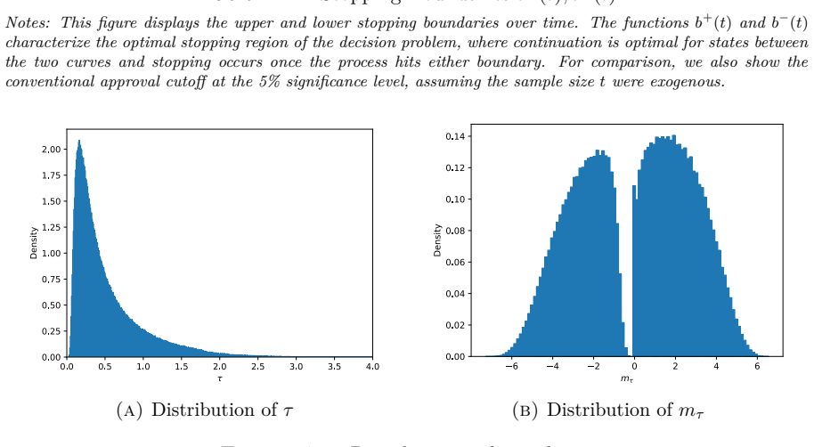
66 (a)0.75V∗ 0 (b)0.9V∗ 0 (c)V ∗ 0 (d)1.01V∗ 0 Figure C.2.Distribution of Posterior Meanm τat Various Values ofV0. C.5.Examination of alternative methods for calibratingBn.In this section, we reproduce the analysis from Section 4.4, but under alternative calibrations forBn. C.5.1.Approval-based benefit.In the first calibration, we setBn = $802million, so ...
work page 2018
-
[14]
The experiment uses fewer samples than in the calibrations withB >0. The reason is that the additional experimentation in the negative region more than offsets the earlier stopping in the positive region. 69 (a)Distribution ofτ (b)Distribution ofm τ Figure C.7.Distributions ofτandm τwhenB n =$0. (a)E[τ∗]vs.V 0/V∗ 0 (b)med[τ∗]vs.V 0/V∗ 0 Figure C.8.The eff...
work page 2022
-
[15]
70 Let cov1 =σ1(˜Σ 11 + ˜Σ 01)and cov0 =σ0(˜Σ 00 + ˜Σ 10)
+ σ0(˜Σ 01 + ˜Σ 00)≥0. 70 Let cov1 =σ1(˜Σ 11 + ˜Σ 01)and cov0 =σ0(˜Σ 00 + ˜Σ 10). Assume without loss of generality that cov1≥cov0, and set t∗:= cov1−cov0 σ0det(˜Σ) . We can characterize the optimal sampling strategy and the resulting posterior variance by employing similar arguments as in Liang et al. (2022, Lemma 11). Theorem 6.Assume that Assumptions 1...
work page 2022
-
[16]
In fact, the majority of the conclusions in Theorem 2 do not depend on the specific form ofmt
The modification of the optimal sampling strategy influences the optimal stopping rule solely via its impact on the quadratic variation ofmt. In fact, the majority of the conclusions in Theorem 2 do not depend on the specific form ofmt. The only step that requires an extra argument is proving thatb+(·)and|b−(·)|are decreasing int. As in the proof of Theor...
work page 2018
discussion (0)
Sign in with ORCID, Apple, or X to comment. Anyone can read and Pith papers without signing in.