Long-Term Clustering Pattern of Solar Active Regions and Their Potential Connection with Magneto-Rossby Waves
Pith reviewed 2026-06-29 20:59 UTC · model grok-4.3
The pith
Three long-term spatiotemporal bands contain over 63% of large solar active region flux and match the phase speeds of slow magneto-Rossby waves with a 4 kG toroidal field.
A machine-rendered reading of the paper's core claim, the machinery that carries it, and where it could break.
Core claim
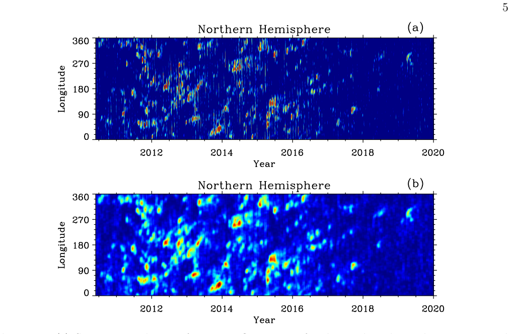
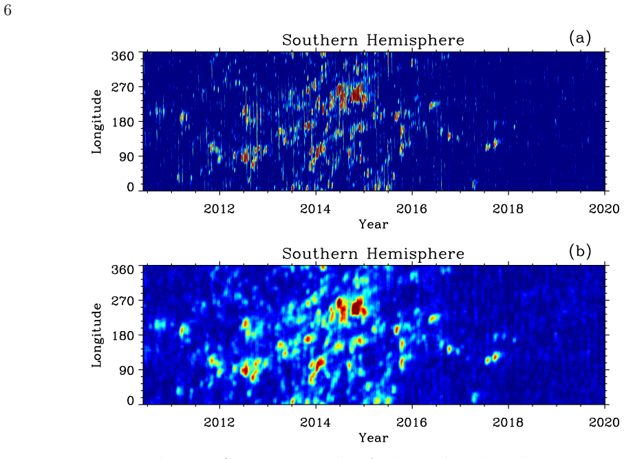
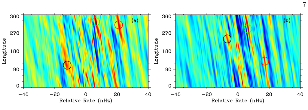
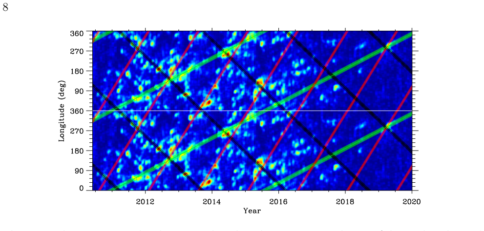
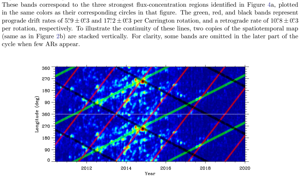
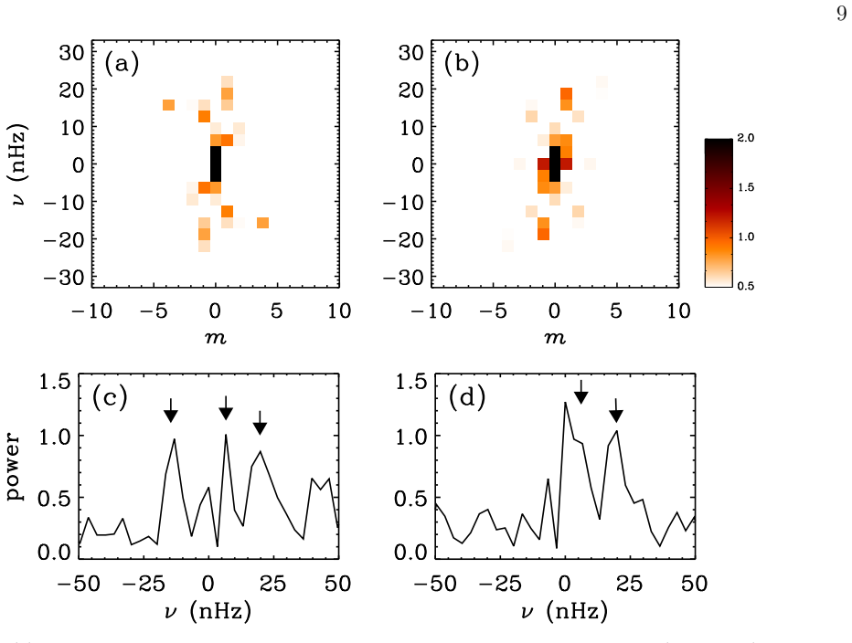
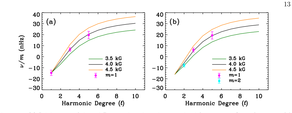
In both hemispheres, over 63% of magnetic fluxes emerge and cluster within or near three distinct bands in the spatiotemporal maps, two of which rotate faster than the Carrington rate and one more slowly. These bands closely correspond to low-order nonaxisymmetric modes, primarily the azimuthal order m=1 mode. The drift rates of the three spatiotemporal bands are in good agreement with the phase speeds inferred for these modes. The frequencies of the dominant modes are consistent with slow magneto-Rossby waves originating in the solar tachocline, associated with odd harmonic degrees ℓ and a toroidal magnetic field strength of approximately 4.0 kG.
What carries the argument
The identification of three observed spatiotemporal clustering bands with the phase speeds and frequencies of low-order (primarily m=1) slow magneto-Rossby wave modes that carry a toroidal field of ~4 kG.
If this is right
- Magneto-Rossby waves modulate both the timing and longitudinal localization of major active region emergence.
- Rieger-type periodicities arise from interactions between a dominant mode and weaker modes.
- Quasi-periodic variations on 0.6-4 yr timescales arise from intersections of multiple major modes.
- Surface magnetic flux patterns connect directly to dynamical processes in the tachocline.
Where Pith is reading between the lines
- If the wave-mode identification holds across cycles, similar clustering bands should appear in earlier or later solar cycles when the same field strength is assumed.
- The model predicts that changes in the internal toroidal field would shift the observed band drift rates in a measurable way.
- Direct comparison of predicted emergence longitudes with new far-side helioseismic maps could test whether the wave mechanism continues to operate.
Load-bearing premise
The three observed spatiotemporal bands correspond to low-order nonaxisymmetric modes (primarily m=1) of slow magneto-Rossby waves whose drift rates and frequencies match those expected for a toroidal field of ~4 kG.
What would settle it
Future maps that show the same three bands persisting but with drift rates or recurrence periods that no longer agree with the phase speeds calculated for slow magneto-Rossby modes at 4 kG would falsify the identification.
Figures
read the original abstract
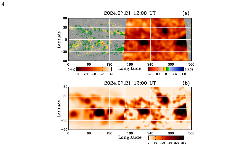
Large solar active regions (ARs) tend to be long lived and spatially clustered, with repeated emergence occurring in persistent solar activity nests over extended timescales. By analyzing long-term spatiotemporal magnetic flux maps constructed from near-side magnetic field observations and far-side helioseismic AR maps, we investigate the recurrence and clustering properties of large ARs during Solar Cycle 24. We find that, in both hemispheres, over 63% of magnetic fluxes emerge and cluster within or near three distinct bands in the spatiotemporal maps, two of which rotate faster than the Carrington rate and one more slowly. These bands closely correspond to low-order nonaxisymmetric modes, primarily the azimuthal order m=1 mode. The drift rates of the three spatiotemporal bands are in good agreement with the phase speeds inferred for these modes. The frequencies of the dominant modes are consistent with slow magneto-Rossby waves originating in the solar tachocline, associated with odd harmonic degrees $\ell$ and a toroidal magnetic field strength of approximately 4.0 kG. Our results suggest that magneto-Rossby waves play an important role in modulating both the timing and longitudinal localization of major AR emergence. Rieger-type periodicities may arise from interactions between a dominant mode and weaker modes, while longer quasi-periodic variations on 0.6--4 yr timescales are likely linked to intersections of multiple major modes. These findings point to a potential connection between surface magnetic flux patterns and dynamical processes in the tachocline.
Editorial analysis
A structured set of objections, weighed in public.
Referee Report
Summary. The paper analyzes long-term spatiotemporal magnetic flux maps from near-side observations and far-side helioseismic AR maps during Solar Cycle 24. It reports that over 63% of the flux emerges and clusters within or near three distinct bands (two prograde and one retrograde relative to the Carrington rate). These bands are identified with low-order nonaxisymmetric modes (primarily m=1) of slow magneto-Rossby waves originating in the tachocline, with odd harmonic degrees ℓ and a toroidal field strength of ~4 kG; the observed drift rates match the theoretical phase speeds, and the frequencies are stated to be consistent with this model. The authors conclude that these waves modulate the timing and longitudinal localization of major AR emergence, with Rieger-type periodicities arising from mode interactions.
Significance. If the mode identification is robust, the result would establish a direct dynamical connection between tachocline magneto-Rossby waves and the observed spatiotemporal clustering of active regions, offering a physical mechanism for both short-term periodicities and longer quasi-periodic variations. The combination of near- and far-side data provides extended longitudinal coverage that strengthens the observational basis. The work builds on prior helioseismic and magnetic-mapping studies but would be strengthened by explicit, reproducible comparison of observed drifts to the dispersion relation.
major comments (3)
- [Abstract] Abstract and § on wave identification: the statement that drift rates 'are in good agreement' with phase speeds for B ≈ 4.0 kG and that frequencies 'are consistent' requires the explicit dispersion relation, the chosen ℓ values, and whether the 4 kG value is an independent prior prediction or obtained by fitting the observed drifts. If the latter, the identification is not secured by the data alone and the causal link to wave modulation is weakened.
- [Results / spatiotemporal maps] The claim that the three bands contain >63% of the flux and 'closely correspond' to m=1 modes needs the precise definition of the bands (e.g., width in longitude and time), the algorithm used to extract them from the flux maps, and a quantitative measure (with uncertainty) of the match between observed drift rates and theoretical phase speeds.
- [Discussion of magneto-Rossby wave model] The assertion that the frequencies match only for odd ℓ and B ~ 4 kG should include the full set of tested (ℓ, m, B) combinations and the χ² or residual values; without this, it is unclear whether other parameter choices could produce comparable agreement.
minor comments (2)
- [Data and methods] Clarify the exact construction of the long-term spatiotemporal maps (binning, interpolation between near- and far-side data, handling of data gaps) so that the 63% flux fraction can be reproduced.
- [Results] Provide the numerical values of the observed drift rates (in deg/day or nHz) alongside the theoretical phase speeds for direct comparison.
Simulated Author's Rebuttal
We thank the referee for the constructive and detailed comments, which highlight areas where additional transparency will improve the manuscript. We agree that explicit details on the dispersion relation, band definitions, and model comparisons are needed. We address each major comment below and will revise the manuscript to incorporate the requested information and quantitative assessments.
read point-by-point responses
-
Referee: [Abstract] Abstract and § on wave identification: the statement that drift rates 'are in good agreement' with phase speeds for B ≈ 4.0 kG and that frequencies 'are consistent' requires the explicit dispersion relation, the chosen ℓ values, and whether the 4 kG value is an independent prior prediction or obtained by fitting the observed drifts. If the latter, the identification is not secured by the data alone and the causal link to wave modulation is weakened.
Authors: We will revise the abstract and relevant sections to include the explicit dispersion relation for slow magneto-Rossby waves. The chosen ℓ values are the odd harmonics (primarily ℓ = 1, 3, 5) for m = 1 modes. The ~4 kG toroidal field is determined by matching the observed drift rates to the theoretical phase speeds; it is not an independent prior. We acknowledge that this fitting approach means the identification relies on the quality of the match rather than a blind prediction. However, the same B value simultaneously reproduces the distinct prograde and retrograde bands, which we view as supporting evidence. The revised text will clarify this and add the dispersion relation with the fitting procedure shown. revision: yes
-
Referee: [Results / spatiotemporal maps] The claim that the three bands contain >63% of the flux and 'closely correspond' to m=1 modes needs the precise definition of the bands (e.g., width in longitude and time), the algorithm used to extract them from the flux maps, and a quantitative measure (with uncertainty) of the match between observed drift rates and theoretical phase speeds.
Authors: We will add precise definitions of the three bands, including their longitudinal widths (approximately ±12–18° depending on the band) and the time spans over which they are tracked. The extraction algorithm is a density-based clustering method applied to the spatiotemporal flux maps with a flux-density threshold; this will be described in the methods section with pseudocode. We will also report quantitative drift-rate comparisons: observed drifts obtained from linear regression to band centroids, with 1σ uncertainties from the fits, compared directly to theoretical phase speeds, including the absolute differences and a statement of agreement within uncertainties. revision: yes
-
Referee: [Discussion of magneto-Rossby wave model] The assertion that the frequencies match only for odd ℓ and B ~ 4 kG should include the full set of tested (ℓ, m, B) combinations and the χ² or residual values; without this, it is unclear whether other parameter choices could produce comparable agreement.
Authors: We will include a new table (or appendix) listing all tested (ℓ, m, B) combinations, covering both even and odd ℓ, m = 1–3, and B values from 1–10 kG. For each we will report the χ² residual between observed and theoretical frequencies/drifts. The table will show that the combination of odd ℓ, m = 1, and B ≈ 4 kG yields the lowest residuals, while other combinations produce substantially larger mismatches. This will be added to the discussion section. revision: yes
Circularity Check
No circularity; wave-mode identification rests on independent dispersion-relation match to observed drifts
full rationale
The paper extracts three spatiotemporal bands containing >63% of flux from observational magnetic maps and helioseismic far-side data, measures their drift rates directly from the data, and reports that these rates agree with phase speeds computed from the slow magneto-Rossby dispersion relation (odd ℓ, m=1) for a tachocline toroidal field of ~4 kG. The 4 kG value is stated as the field strength that produces consistency, not as a parameter fitted inside the present analysis and then relabeled a prediction. No equation in the provided text defines a quantity in terms of itself, renames a fit as a first-principles result, or imports a uniqueness theorem solely via self-citation. The derivation chain therefore remains self-contained against external benchmarks and receives the default non-circularity finding.
Axiom & Free-Parameter Ledger
free parameters (1)
- toroidal magnetic field strength =
4.0 kG
axioms (2)
- domain assumption The three spatiotemporal bands correspond to low-order nonaxisymmetric magneto-Rossby wave modes with m=1
- domain assumption The waves originate in the solar tachocline
Reference graph
Works this paper leans on
-
[1]
2003, ApJ, 585, 1114, doi: 10.1086/346152
Bai, T. 2003, ApJ, 585, 1114, doi: 10.1086/346152
-
[2]
Bai, T., & Sturrock, P. A. 1987, Nature, 327, 601, doi: 10.1038/327601a0
-
[3]
Baldner, C. S., & Basu, S. 2008, ApJ, 686, 1349, doi: 10.1086/591514
-
[4]
Bazilevskaya, G., Broomhall, A.-M., Elsworth, Y., & Nakariakov, V. M. 2014, SSRv, 186, 359, doi: 10.1007/s11214-014-0068-0
-
[5]
Scherrer, P. H. 1999, SoPh, 190, 145, doi: 10.1023/A:1005270318209
-
[6]
Berdyugina, S. V., & Usoskin, I. G. 2003, A&A, 405, 1121, doi: 10.1051/0004-6361:20030748
-
[7]
Bogart, R. S. 1982, SoPh, 76, 155, doi: 10.1007/BF00214137
-
[8]
Bogart, R. S., & Bai, T. 1985, ApJL, 299, L51, doi: 10.1086/184579
-
[9]
2005, PhR, 417, 1, doi: 10.1016/j.physrep.2005.06.005
Brandenburg, A., & Subramanian, K. 2005, PhR, 417, 1, doi: 10.1016/j.physrep.2005.06.005
-
[10]
1969, SoPh, 7, 28, doi: 10.1007/BF00148402
Bumba, V., & Howard, R. 1969, SoPh, 7, 28, doi: 10.1007/BF00148402
-
[11]
Zalm, E. B. J. 1986, SoPh, 105, 237, doi: 10.1007/BF00172045
-
[12]
2022, ApJ, 941, 197, doi: 10.3847/1538-4357/aca333
Chen, R., Zhao, J., Hess Webber, S., et al. 2022, ApJ, 941, 197, doi: 10.3847/1538-4357/aca333
-
[13]
2002, ApJL, 578, L157, doi: 10.1086/344635 16 de Toma, G., White, O
Chou, D.-Y., & Serebryanskiy, A. 2002, ApJL, 578, L157, doi: 10.1086/344635 16 de Toma, G., White, O. R., & Harvey, K. L. 2000, ApJ, 529, 1101, doi: 10.1086/308299
-
[14]
McIntosh, S. W. 2018a, ApJ, 862, 159, doi: 10.3847/1538-4357/aacefa
-
[15]
Dikpati, M., McIntosh, S. W., Bothun, G., et al. 2018b, ApJ, 853, 144, doi: 10.3847/1538-4357/aaa70d
-
[16]
Dikpati, M., McIntosh, S. W., Chatterjee, S., et al. 2021, ApJ, 910, 91, doi: 10.3847/1538-4357/abe043
-
[17]
2021, Living Reviews in Solar Physics, 18, 5, doi: 10.1007/s41116-021-00031-2
Fan, Y. 2021, Living Reviews in Solar Physics, 18, 5, doi: 10.1007/s41116-021-00031-2
-
[18]
Gilman, P. A. 1969, SoPh, 8, 316, doi: 10.1007/BF00155379
-
[19]
2000, Science, 287, 2456, doi: 10.1126/science.287.5462.2456
Howe, R., Christensen-Dalsgaard, J., Hill, F., et al. 2000, Science, 287, 2456, doi: 10.1126/science.287.5462.2456
-
[20]
Jain, K., Chowdhury, P., & Tripathy, S. C. 2023, ApJ, 959, 16, doi: 10.3847/1538-4357/ad045c Kors´ os, M. B., Dikpati, M., Erd´ elyi, R., Liu, J., &
-
[21]
2023, ApJ, 944, 180, doi: 10.3847/1538-4357/acb64f
Zuccarello, F. 2023, ApJ, 944, 180, doi: 10.3847/1538-4357/acb64f
-
[22]
Krista, L. D., McIntosh, S. W., & Leamon, R. J. 2018, AJ, 155, 153, doi: 10.3847/1538-3881/aaaebf
-
[23]
1990, ApJ, 363, 718, doi: 10.1086/169378
Lean, J. 1990, ApJ, 363, 718, doi: 10.1086/169378
-
[24]
Liang, Z.-C., Gizon, L., Birch, A. C., & Duvall, T. L. 2019, A&A, 626, A3, doi: 10.1051/0004-6361/201834849 L¨ optien, B., Gizon, L., Birch, A. C., et al. 2018, Nature Astronomy, 2, 568, doi: 10.1038/s41550-018-0460-x
-
[25]
2000, ApJ, 540, 1102, doi: 10.1086/309387
Lou, Y.-Q. 2000, ApJ, 540, 1102, doi: 10.1086/309387
-
[26]
Wang, J. X. 2003, MNRAS, 345, 809, doi: 10.1046/j.1365-8711.2003.06993.x
-
[27]
Marcano, M., & Leamon, R. J. 2017, Nature Astronomy, 1, 0086, doi: 10.1038/s41550-017-0086
-
[28]
Moderate Nesting and Cross-Equatorial Asymmetry of Active Regions in Solar Cycle 24
Raj, A. 2025, arXiv e-prints, arXiv:2511.03646, doi: 10.48550/arXiv.2511.03646
work page internal anchor Pith review Pith/arXiv arXiv doi:10.48550/arxiv.2511.03646 2025
-
[29]
Pesnell, W. D., Thompson, B. J., & Chamberlin, P. C. 2012, SoPh, 275, 3, doi: 10.1007/s11207-011-9841-3
-
[30]
Teruya, A. S. W. 2024, A&A, 692, A102, doi: 10.1051/0004-6361/202451014
-
[31]
Raphaldini, B., Dikpati, M., & McIntosh, S. W. 2023, ApJ, 953, 156, doi: 10.3847/1538-4357/ace320
-
[32]
2006, ApJ, 647, 662, doi: 10.1086/505170
Rempel, M. 2006, ApJ, 647, 662, doi: 10.1086/505170
-
[33]
Rieger, E., Share, G. H., Forrest, D. J., et al. 1984, Nature, 312, 623, doi: 10.1038/312623a0
-
[34]
Smith, E. J. 2001, J. Geophys. Res., 106, 8363, doi: 10.1029/2000JA000392
-
[35]
Scherrer, P. H., Schou, J., Bush, R. I., et al. 2012, SoPh, 275, 207, doi: 10.1007/s11207-011-9834-2
-
[36]
Schou, J., Scherrer, P. H., Bush, R. I., et al. 2012, SoPh, 275, 229, doi: 10.1007/s11207-011-9842-2
-
[37]
2012, ApJ, 749, 27, doi: 10.1088/0004-637X/749/1/27
Vecchio, A., Laurenza, M., Meduri, D., Carbone, V., & Storini, M. 2012, ApJ, 749, 27, doi: 10.1088/0004-637X/749/1/27
-
[38]
2023, ApJL, 954, L26, doi: 10.3847/2041-8213/acefd0
Waidele, M., & Zhao, J. 2023, ApJL, 954, L26, doi: 10.3847/2041-8213/acefd0
-
[39]
Xiang, N. B., Zhao, X. H., & Li, F. Y. 2021, PASA, 38, e032, doi: 10.1017/pasa.2021.30
-
[40]
Ballester, J. L. 2010a, ApJ, 709, 749, doi: 10.1088/0004-637X/709/2/749 —. 2010b, ApJL, 724, L95, doi: 10.1088/2041-8205/724/1/L95
-
[41]
Zaqarashvili, T. V., & Gurgenashvili, E. 2018, Frontiers in Astronomy and Space Sciences, 5, 7, doi: 10.3389/fspas.2018.00007
-
[42]
Shergelashvili, B. M. 2007, A&A, 470, 815, doi: 10.1051/0004-6361:20077382
-
[43]
2019, ApJ, 887, 216, doi: 10.3847/1538-4357/ab5951
Zhao, J., Hing, D., Chen, R., & Hess Webber, S. 2019, ApJ, 887, 216, doi: 10.3847/1538-4357/ab5951
discussion (0)
Sign in with ORCID, Apple, or X to comment. Anyone can read and Pith papers without signing in.