Rapid Approximation Prediction for Kriging
Pith reviewed 2026-06-29 06:18 UTC · model grok-4.3
The pith
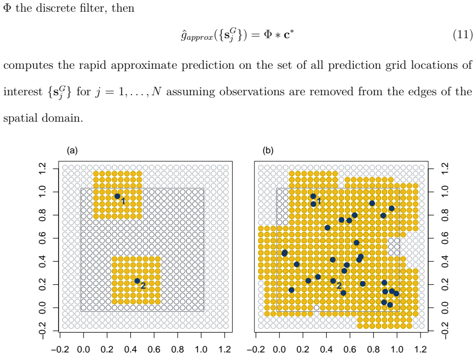
Kriging prediction on regular grids is reformulated by approximating each off-grid covariance vector as a sparse linear combination of M on-grid covariances from a local neighborhood, cutting complexity from O(N n^3) to O(N log N + nM + M^3
A machine-rendered reading of the paper's core claim, the machinery that carries it, and where it could break.
Core claim
By approximating each off-grid covariance vector by a sparse linear combination of on-grid covariances within a local L-order neighborhood of M = (2L)^2 neighboring grid points, the reformulation reduces complexity from O(N n^3) to O(N log N + nM + M^3) while preserving accuracy for stationary Gaussian processes on regular prediction grids.
What carries the argument
Sparse linear combination of M = (2L)^2 on-grid covariances that approximates each off-grid covariance vector inside a local L-order neighborhood.
If this is right
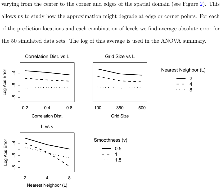
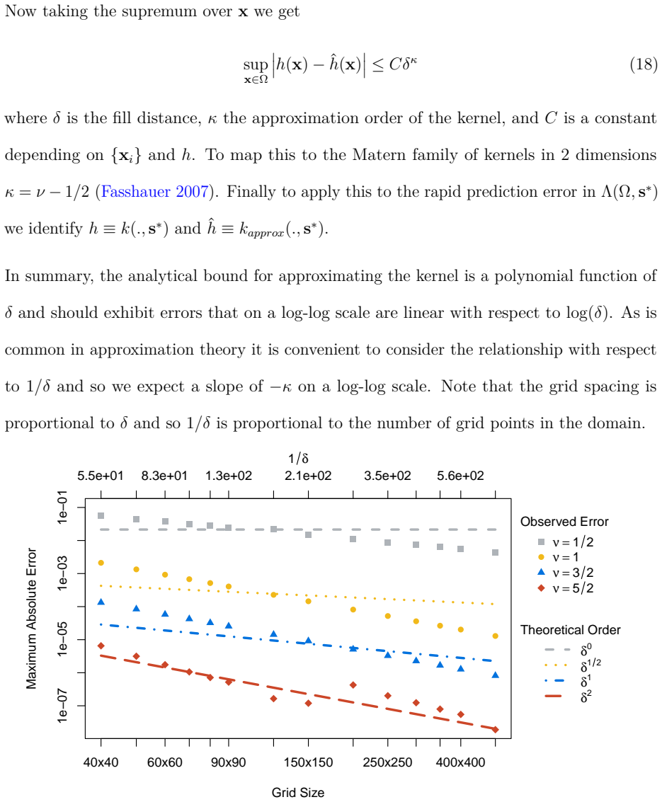
- Approximation error decreases systematically as Matérn smoothness increases, neighbor order L increases, or grid resolution increases.
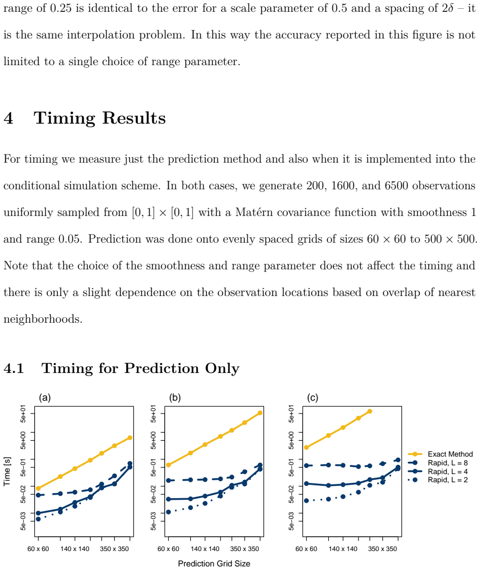
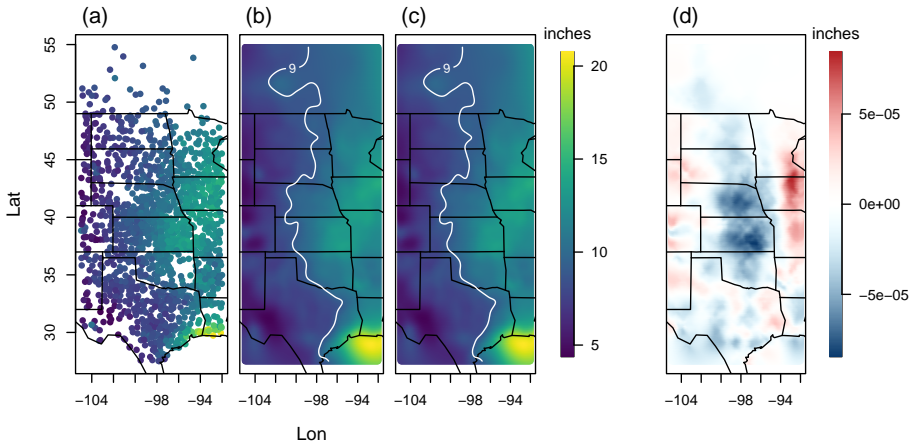
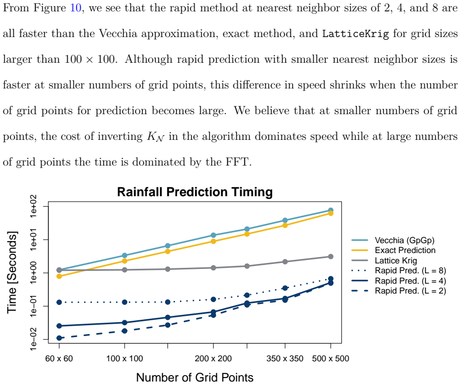
- At n=1368 and a 350 by 350 prediction grid the method yields pointwise errors on the order of 10^{-5} inches and more than 150 times speedup over exact Kriging.
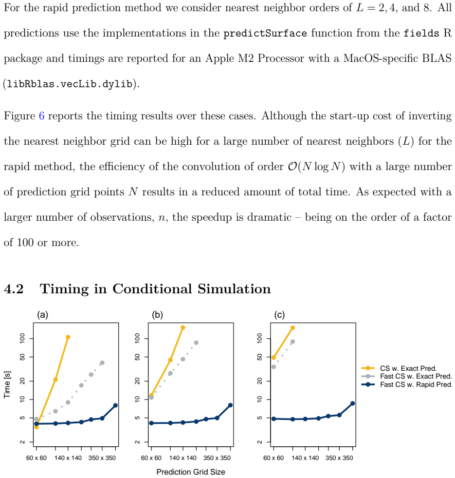
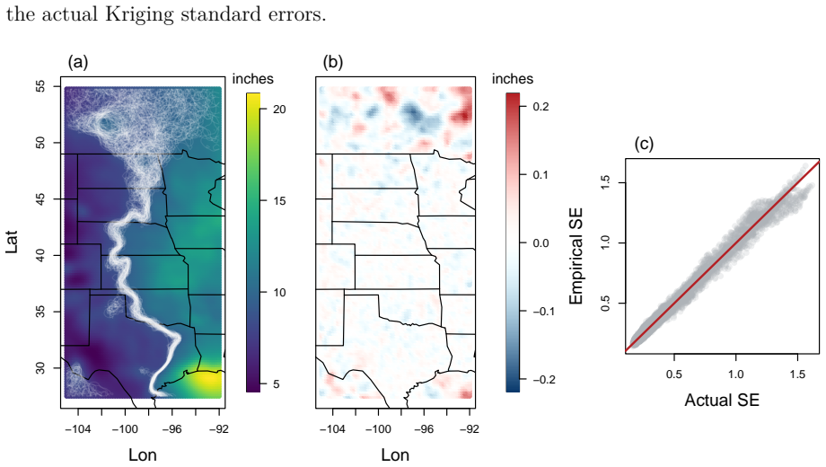
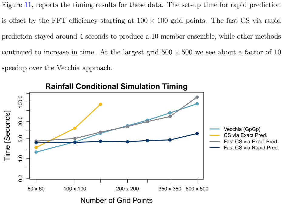
- When embedded inside a fast conditional-simulation scheme the approximation reproduces the exact Kriging standard-error field and continues to scale with both n and N.
- The method outperforms Vecchia and LatticeKrig approximations on the rainfall mapping task while remaining compatible with a two-stage workflow of fast parameter estimation followed by rapid fine-grid prediction.
Where Pith is reading between the lines
- The same neighborhood construction could be tested on non-stationary covariance functions to determine where the stationarity assumption becomes the limiting factor.
- Because the dominant cost is now linear in grid size, the approach opens the possibility of routine uncertainty quantification on continental-scale grids that are currently handled only by simplified models.
- Replacing the fixed rectangular neighborhood with an adaptive selection of M points might further reduce error on irregularly spaced observation sets without changing the overall complexity scaling.
Load-bearing premise
Each off-grid covariance vector can be approximated by a sparse linear combination of on-grid covariances within a local L-order neighborhood of M = (2L)^2 neighboring grid points.
What would settle it
Compute exact versus approximated Kriging predictions on the North American summer-rainfall data set (n=1368) at a 350 by 350 grid for L=2 and Matérn smoothness 1.5; if the maximum pointwise absolute error exceeds 10^{-4} inches the central accuracy claim is falsified.
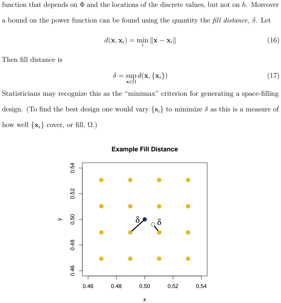
Figures
read the original abstract
Exact Kriging and conditional simulation (CS) for uncertainty quantification are computationally infeasible for modern spatial analyses with large numbers of observations and dense prediction grids. We present a rapid approximation to the Kriging prediction step for stationary Gaussian processes for a regular prediction grid by approximating each off-grid covariance vector by a sparse linear combination of on-grid covariances within a local $L$-order neighborhood of $M = (2L)^2$ neighboring grid points. This reformulation reduces complexity from $O(N n^3)$ to $O(N \log N + nM + M^3)$ while preserving accuracy. A factorial study shows that approximation error decreases systematically with increased Mat\'{e}rn smoothness, neighbor order $L$, and grid resolution, aligning with bounds from kernel approximation theory. In a North American summer-rainfall application ($n=1368$), our method produces predictions visually indistinguishable from exact Kriging with point-wise errors on the order of $10^{-5}$ inches and achieves more than $150$ times speedups at a $350\times350$ grid, also outperforming Vecchia and LatticeKrig predictions. Embedded in a fast CS scheme, the approach reproduces Kriging standard errors and scales favorably with both $n$ and $N$. We recommend a practical workflow that uses a fast method for parameter estimation followed by our rapid predictor for fine-grid mapping and uncertainty quantification.
Editorial analysis
A structured set of objections, weighed in public.
Referee Report
Summary. The manuscript presents a rapid approximation for the Kriging prediction step (and conditional simulation) for stationary Gaussian processes on regular grids. Each off-grid covariance vector of length n is approximated as a sparse linear combination of M=(2L)^2 on-grid covariance vectors drawn from a local L-order neighborhood. The authors claim this reduces complexity from O(N n^3) to O(N log N + nM + M^3) while preserving accuracy, supported by a factorial simulation study showing systematic error reduction with Matérn smoothness, L, and grid resolution, plus a real-data example (n=1368 North American rainfall observations) yielding 10^{-5}-level pointwise errors, >150x speedups on a 350×350 grid, and better performance than Vecchia and LatticeKrig approximations.
Significance. If the complexity bound holds without hidden per-prediction costs and the accuracy claims are substantiated, the method would provide a practical, scalable tool for fine-grid spatial prediction and uncertainty quantification that outperforms several existing approximations in the reported application. The alignment of empirical error behavior with kernel approximation theory and the embedded fast CS scheme are positive features.
major comments (2)
- [Abstract] Abstract (complexity claim): The stated reduction to O(N log N + nM + M^3) is central to the paper's contribution. The construction requires, for each of the N distinct prediction locations, solving the local M×M system K_MM a = k_M(x) to obtain the combination coefficients; absent a global fast transform or translation-invariant stencil (neither mentioned in the abstract or the high-level description), this step contributes an O(N M^3) term. The published bound therefore appears incomplete and must be justified or revised with an explicit accounting of the coefficient solve cost.
- [Factorial study / real-data application] Factorial study and real-data section: The claim that approximation error decreases systematically with Matérn smoothness, neighbor order L, and grid resolution is load-bearing for the accuracy-preservation argument. The manuscript reports 10^{-5} errors and visual indistinguishability but provides no visible derivation details, explicit a priori error bounds, or quantitative comparison against the kernel approximation theory bounds invoked; without these, it is difficult to assess whether the observed rates are consistent with the theoretical expectations or merely empirical.
minor comments (2)
- [Abstract] Notation for n (observation count) and N (prediction locations) should be defined at first use rather than left implicit in the complexity expressions.
- [Abstract] The abstract states the method 'outperforms Vecchia and LatticeKrig predictions' but does not specify the exact metrics or settings (e.g., same L or equivalent computational budget) used for the comparison; a brief clarification would improve reproducibility.
Simulated Author's Rebuttal
We thank the referee for the careful reading and constructive comments on our manuscript. We address the two major comments point by point below and will revise the paper to incorporate the necessary clarifications and additions.
read point-by-point responses
-
Referee: [Abstract] Abstract (complexity claim): The stated reduction to O(N log N + nM + M^3) is central to the paper's contribution. The construction requires, for each of the N distinct prediction locations, solving the local M×M system K_MM a = k_M(x) to obtain the combination coefficients; absent a global fast transform or translation-invariant stencil (neither mentioned in the abstract or the high-level description), this step contributes an O(N M^3) term. The published bound therefore appears incomplete and must be justified or revised with an explicit accounting of the coefficient solve cost.
Authors: We agree the stated bound is incomplete as written. Because the process is stationary and the grid is regular, every local L-order neighborhood has an identical relative configuration; thus K_MM is translation-invariant and can be factored once in O(M^3) time. Each of the N coefficient vectors is then obtained by an O(M^2) solve with the precomputed factor. The original expression therefore omitted the resulting O(N M^2) term. We will revise the abstract and the complexity discussion to read O(N M^2 + N log N + nM + M^3) and will explicitly note the translation-invariant stencil and one-time precomputation. revision: yes
-
Referee: [Factorial study / real-data application] Factorial study and real-data section: The claim that approximation error decreases systematically with Matérn smoothness, neighbor order L, and grid resolution is load-bearing for the accuracy-preservation argument. The manuscript reports 10^{-5} errors and visual indistinguishability but provides no visible derivation details, explicit a priori error bounds, or quantitative comparison against the kernel approximation theory bounds invoked; without these, it is difficult to assess whether the observed rates are consistent with the theoretical expectations or merely empirical.
Authors: We accept that the manuscript would be strengthened by making the link to kernel approximation theory explicit. In revision we will add a short subsection that (i) recalls the relevant a priori bounds on the covariance-function approximation error, (ii) derives the expected scaling of the pointwise Kriging error with Matérn smoothness ν, neighborhood order L, and grid spacing, and (iii) overlays the empirical error curves obtained in the factorial study against these theoretical rates. This will demonstrate that the observed 10^{-5}-level errors and their systematic dependence are consistent with theory rather than purely empirical. revision: yes
Circularity Check
No circularity; derivation is self-contained from local covariance construction
full rationale
The paper defines the approximation explicitly as each off-grid covariance vector being a sparse linear combination of M on-grid vectors within a local L-order neighborhood, then states the resulting complexity as O(N log N + nM + M^3) from that reformulation. No step reduces by construction to a fitted parameter renamed as prediction, a self-citation chain, or an ansatz smuggled from prior work by the same authors. Accuracy claims are supported by factorial studies and external application data rather than internal redefinition. The central claims remain independent of the inputs they are derived from.
Axiom & Free-Parameter Ledger
free parameters (1)
- L (neighbor order)
axioms (1)
- domain assumption The random field is a stationary Gaussian process
Reference graph
Works this paper leans on
-
[1]
D., Bandyopadhyay, S
Bailey, M. D., Bandyopadhyay, S. & Nychka, D. (2022), ‘Adapting conditional simulation using circulant embedding for irregularly spaced spatial data’,Stat11
2022
-
[2]
Fasshauer, G. E. (2006), Meshfree methods,inM. Rieth & W. Schommers, eds, ‘Handbook of Theoretical and Computational Nanotechnology’, Vol. 2, American Scientific Publishers, pp. 33–97
2006
-
[3]
Fasshauer, G. E. (2007),Meshfree approximation methods with MATLAB, World Scientific
2007
-
[4]
& Fahmy, Y
Guinness, J., Katzfuss, M. & Fahmy, Y. (2024),GpGp: Fast Gaussian Process Computation Using Vecchia’s Approximation. R package version 0.5.1. URL:https://cran.r-project.org/package=GpGp
2024
- [5]
-
[6]
(1952), ‘A statistical approach to some basic mine valuation problems on the witwatersrand, by d.g
Krige, D. (1952), ‘A statistical approach to some basic mine valuation problems on the witwatersrand, by d.g. krige, published in the journal, december 1951 : introduction by the author’,Journal of the South African Institute of Mining and Metallurgy52(9), 201–203
1952
-
[7]
Lindgren, F., Rue, H. & Lindström, J. (2011), ‘An explicit link between gaussian fields and gaussian markov random fields: the stochastic partial differential equation approach’, Journal of the Royal Statistical Society: Series B (Statistical Methodology)73(4), 423–498. URL:https://rss.onlinelibrary.wiley.com/doi/abs/10.1111/j.1467-9868.2011.00777.x
-
[8]
(1965),Les Variables Régionalisées et leur estimation: Une Application de la Théorie des Fonctions Aléatoires aux Sciences de la Nature, Paris, Masson et Cie
Matheron, G. (1965),Les Variables Régionalisées et leur estimation: Une Application de la Théorie des Fonctions Aléatoires aux Sciences de la Nature, Paris, Masson et Cie. 37
1965
-
[9]
& Johnson, R
Nychka, D., Furrer, R., Paige, J., Sain, S., Gerber, F., Iverson, M. & Johnson, R. (2025), fields: Tools for Spatial Data. R package version 17.1. URL:https://cran.r-project.org/package=fields
2025
-
[10]
& Sikorski, A
Nychka, D., Hammerling, D., Sain, S., Lenssen, N., Smirniotis, C., Iverson, M. & Sikorski, A. (2024),LatticeKrig: Multi-Resolution Kriging Based on Markov Random Fields. R package version 9.3.0. URL:https://cran.r-project.org/package=LatticeKrig
2024
-
[11]
Stein, M. L. (2011), ‘2010 Rietz Lecture: When does the screening effect hold?’,The Annals of Statistics39(6). URL:http://dx.doi.org/10.1214/11-AOS909
-
[12]
Tobler, W. R. (1970), ‘A computer movie simulating urban growth in the detroit region’, Economic Geography46, 234–240. URL:http://www.jstor.org/stable/143141
1970
-
[13]
Wu, Z.-M. & Schaback, R. (1993), ‘Local error estimates for radial basis function interpola- tion of scattered data’,IMA Journal of Numerical Analysis13(1), 13–27. URL:https://doi.org/10.1093/imanum/13.1.13 38
discussion (0)
Sign in with ORCID, Apple, or X to comment. Anyone can read and Pith papers without signing in.