Efficient Inference for Incremental Causal Effects of Time to Treatment
Pith reviewed 2026-06-29 06:15 UTC · model grok-4.3
The pith
The efficient influence function for incremental causal effects of time-to-treatment intensity supports machine learning estimation with fast rates.
A machine-rendered reading of the paper's core claim, the machinery that carries it, and where it could break.
Core claim
We derive the efficient influence function for the incremental causal effect of intervening on the intensity of time to treatment initiation. This enables a framework for estimation using machine learning methods that achieves fast convergence rates, with valid confidence bands obtained via empirical process theory.
What carries the argument
Efficient influence function for the incremental causal effect of continuous-time intervention on treatment intensity
If this is right
- Flexible machine learning can be used for estimation without losing fast rates.
- Valid confidence intervals are available for these effects.
- The approach can be used in applications like disease screening to study effects on health outcomes.
- Simulations confirm the method's performance under the stated conditions.
Where Pith is reading between the lines
- Similar methods could apply to other continuous-time causal estimands in medical research.
- Changing screening policies might be evaluated through such incremental intensity effects.
- Extensions to multiple treatments or competing risks could build on this EIF derivation.
Load-bearing premise
The efficient influence function for the incremental causal effect exists and meets the regularity conditions needed for the fast convergence and valid inference.
What would settle it
Observing that the proposed estimator's convergence rate is slower than claimed or that the confidence bands have incorrect coverage in a setting satisfying the paper's assumptions would falsify the claims.
Figures
read the original abstract
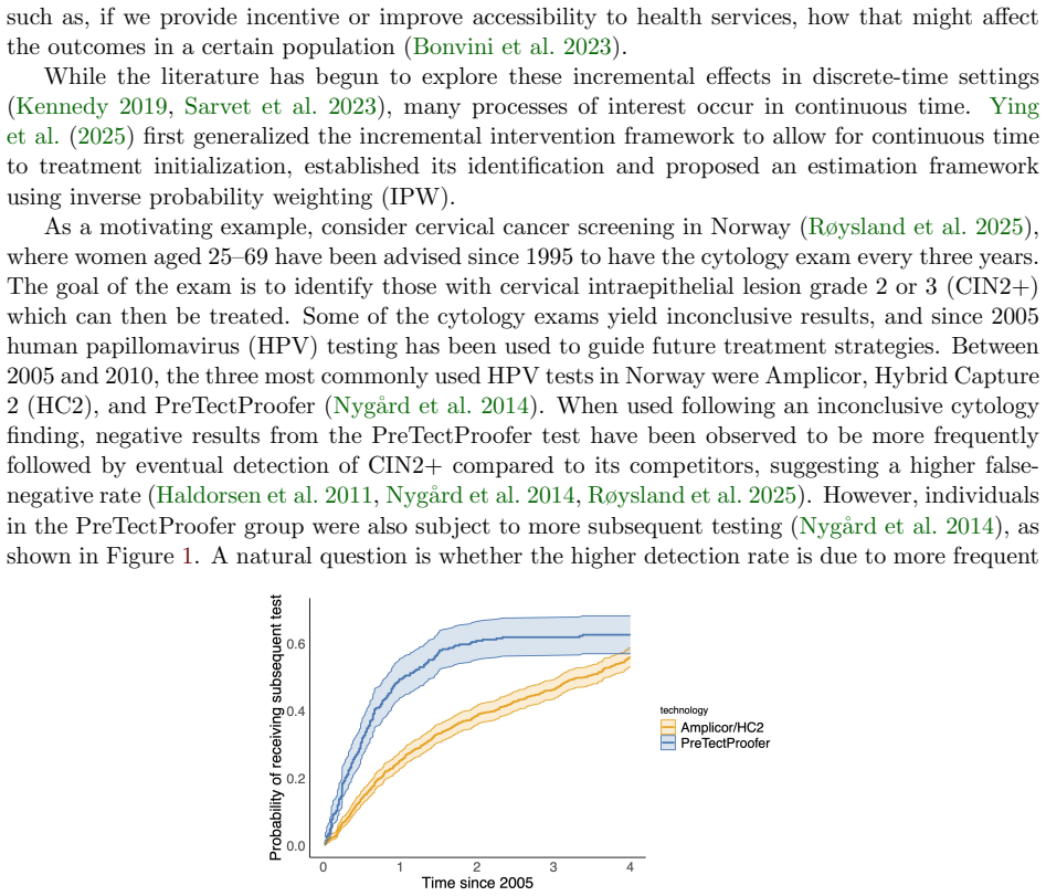
We consider continuous time to treatment initiation. This can commonly occur in preventive medicine, such as disease screening and vaccination; it can also occur with non-fatal health conditions such as HIV infection without the onset of AIDS. While traditional causal inference focused on `when to treat' and its effects, we consider the incremental causal effect when the intensity of time to treatment initiation is intervened upon. We derive the efficient influence function for this estimand and develop an estimation framework that accommodates flexible machine learning methods while achieving fast convergence rates. Valid confidence bands are obtained leveraging empirical process theory. We illustrate our approach via simulation, and apply it to cervical cancer screening data to study the incremental effect of time to subsequent HPV testing on cervical intraepithelial neoplasia detection.
Editorial analysis
A structured set of objections, weighed in public.
Referee Report
Summary. The paper considers continuous-time interventions on the intensity of time-to-treatment initiation and defines an incremental causal effect estimand for this setting. It derives the efficient influence function (EIF) for the estimand, constructs an estimator that accommodates machine learning for nuisance functions while targeting fast convergence rates, and obtains valid confidence bands via empirical process theory. The method is evaluated in simulations and applied to cervical cancer screening data to assess the effect of HPV testing intensity on neoplasia detection.
Significance. If the EIF derivation and rate results hold under the maintained regularity conditions, the work would provide a practically useful extension of efficient causal estimation to continuous-time intensity interventions, a setting common in preventive medicine. The explicit accommodation of flexible ML estimators together with empirical-process-based inference is a methodological strength that could support reproducible applications in observational health data.
major comments (3)
- [§3.2] §3.2, Assumption 3 (positivity): the stated boundedness-away-from-zero condition on the intensity process is invoked to guarantee existence of the EIF and the Donsker property needed for the n^{-1/2} rate, yet the paper provides no diagnostic or sensitivity analysis showing that this condition is plausible for the time-to-treatment intensity in the cervical screening application or in the simulation designs.
- [§4.1] §4.1, Theorem 1: the proof that the EIF yields the claimed semiparametric efficiency bound relies on the intensity process satisfying sufficient smoothness for the relevant function classes to have controlled entropy; without explicit verification or additional regularity assumptions on the compensator, the fast-rate claim cannot be assessed from the given derivation.
- [§5.3] §5.3, simulation design: the reported coverage of the confidence bands is close to nominal only under the simulated intensities that are artificially bounded away from zero; it is unclear whether the same coverage holds when the intensity process is allowed to hit zero on positive-measure sets, which is the more realistic case for time-to-treatment data.
minor comments (2)
- [§2] Notation for the intensity process and the intervention parameter is introduced in §2 but reused with slight variations in §3; a single consolidated definition table would improve readability.
- [§6] The application section reports point estimates and bands but does not include a table of the estimated nuisance functions or their convergence diagnostics, which would help readers assess whether the ML components satisfied the rate conditions used in the theory.
Simulated Author's Rebuttal
We thank the referee for the constructive and detailed comments. We address each major comment below and propose revisions where appropriate to strengthen the manuscript.
read point-by-point responses
-
Referee: [§3.2] §3.2, Assumption 3 (positivity): the stated boundedness-away-from-zero condition on the intensity process is invoked to guarantee existence of the EIF and the Donsker property needed for the n^{-1/2} rate, yet the paper provides no diagnostic or sensitivity analysis showing that this condition is plausible for the time-to-treatment intensity in the cervical screening application or in the simulation designs.
Authors: We agree that explicit diagnostics would strengthen the presentation. In the revision we will add plots of the fitted intensity processes from both the simulation designs and the cervical screening application, confirming they remain bounded away from zero on the relevant support. We will also include a sensitivity analysis that varies the lower bound and reports the resulting changes to the incremental effect estimates. revision: yes
-
Referee: [§4.1] §4.1, Theorem 1: the proof that the EIF yields the claimed semiparametric efficiency bound relies on the intensity process satisfying sufficient smoothness for the relevant function classes to have controlled entropy; without explicit verification or additional regularity assumptions on the compensator, the fast-rate claim cannot be assessed from the given derivation.
Authors: Theorem 1 is derived under the maintained regularity conditions that the compensator is Lipschitz continuous, which ensures the relevant function classes are Donsker with controlled entropy. We will revise the statement of Theorem 1 to list these conditions explicitly and add a short remark justifying their plausibility for intensity processes arising in survival data. revision: yes
-
Referee: [§5.3] §5.3, simulation design: the reported coverage of the confidence bands is close to nominal only under the simulated intensities that are artificially bounded away from zero; it is unclear whether the same coverage holds when the intensity process is allowed to hit zero on positive-measure sets, which is the more realistic case for time-to-treatment data.
Authors: The positivity assumption (Assumption 3) is required for the EIF to exist and for the n^{-1/2} rate to hold; simulations that allow the intensity to hit zero would fall outside the theorem's scope. We will add a clarifying paragraph in §5.3 and an additional simulation scenario in which the intensity approaches but does not reach zero, illustrating the gradual loss of coverage as the bound tightens. revision: partial
Circularity Check
No circularity: derivation presented as independent EIF construction
full rationale
The abstract states that the EIF for the incremental causal effect under continuous-time intensity intervention is derived, with estimation and rates obtained via machine learning and empirical process theory. No equations, self-citations, or steps are provided that reduce the claimed EIF or convergence rates to a fitted input, self-defined quantity, or load-bearing prior result by the same authors. The central claim remains a standard derivation from the observed data law and intervention, self-contained against external semiparametric theory without the reductions enumerated in the circularity patterns.
Axiom & Free-Parameter Ledger
Reference graph
Works this paper leans on
-
[1]
Andersen, P. K. & Gill, R. D. (1982), ‘Cox’s regression model for counting processes: A large sample study’,The Annals of Statistics10(4), 1100–1120. Apostol, T. M. (1974),Mathematical analysis, Addison-Wesley. Athey, S., Tibshirani, J. & Wager, S. (2019), ‘Generalized random forests’,The Annals of Statistics 47(2), 1148–1178. Belloni, A., Chernozhukov, V...
1982
-
[2]
(1923), ‘Sur les applications de la th´ eorie des probabilit´ es aux experiences agricoles: Essai des principes’,Roczniki Nauk Rolniczych10(1), 1–51
Neyman, J. (1923), ‘Sur les applications de la th´ eorie des probabilit´ es aux experiences agricoles: Essai des principes’,Roczniki Nauk Rolniczych10(1), 1–51. Nyg˚ ard, M., Røysland, K., Campbell, S. & Dillner, J. (2014), ‘Comparative effectiveness study on human papillomavirus detection methods used in the cervical cancer screening programme’,BMJ Open4...
1923
-
[3]
Ying, A. (2024), ‘Causality for complex continuous-time functional longitudinal studies with dy- namic treatment regimes’,arXiv preprint arXiv:2406.06868. Ying, A., Zhao, Z. & Xu, R. (2025), Incremental causal effect for time to treatment initialization, inY. Yue, A. Garg, N. Peng, F. Sha & R. Yu, eds, ‘International Conference on Learning Representations...
-
[4]
Z ˜u∧u 0 {θ(v, ˜l)−1} S(v|˜l) dΛ0(v|˜l) # f(y|u, ˜l)f(u|˜l)dydu = Z E(Y|u, ˜l)θ(u, ˜l)δe− R u 0 {θ(v,˜l)−1}dΛ0(v|˜l) Z ˜u∧u 0 {θ(v, ˜l)−1} S(v|˜l) dΛ0(v|˜l)f(u|˜l)du =E
In (S1), using the upper limitU−ensures that individuals treated exactly atτare classified as untreated, and is essential to correctly derive the efficient influence function in the presence of a point mass at τ. Since the cumulative hazard functions ofUandTgivenLare identical on [0, τ), we interpret Λ0(v|L) ing(O,P) as the cumulative hazard function ofUa...
2022
-
[5]
This integral admits integration by parts in the form R b a f(x)dg(x) =f(b)g(b)−f(a)g(a)− R b a g(x)d f(x) (Apostol 1974)
We will use the fact that the Riemann–Stieltjes integral R b a f(x)dg(x) exists if bothfandgare of bounded variation and share no common discontinuities (Young 1936). This integral admits integration by parts in the form R b a f(x)dg(x) =f(b)g(b)−f(a)g(a)− R b a g(x)d f(x) (Apostol 1974). First, under Assumption 3, we have the bound e ˆΛ(t|l) −e Λ0(t|l) ≤...
1936
-
[6]
In the following for a random functionX(t, l) witht∈[0, τ] andl∈ L, define∥X(·, L)∥ 2 sup,2 = E{supt∈[0,τ] |X(t, L)|2}and∥X(·, L)∥ 2 TV,2 =E TV{X(·, L)}2 . Assumption S2.Suppose that ∥R2(·, L)∥sup,2 =o(n −1/2),∥ ˜R1(·, L)∥sup,2 =o(n −1/2),∥ ˜R1(·, L)∥TV,2 =O(1), ∥ ˜R2(·, L)∥sup,2 =o(n −1/2),∥ ˜R3(·, L)∥sup,2 =o(n −1/2), and ∥R2(·, L) ˜R2(·, L)∥sup,2 =o(n ...
1972
-
[7]
Assumption S3 is a integrability condition on the product of integrals involving the influence functions of the RAL estimators, and is also similarly assumed in Wang et al
The conditions for the product remainder terms can also be satisfied; for example, when one remainder term is almost surely bounded and the other converges at rate n−1/2. Assumption S3 is a integrability condition on the product of integrals involving the influence functions of the RAL estimators, and is also similarly assumed in Wang et al. (2024). Proof...
2024
-
[8]
33 Let|J |denote the cardinality ofJ. Then |J |= 4 1 n(n−1) 5 − 4 2 n(n−1)(n−2) 4 + 4 3 n(n−1)(n−2)(n−3) 3 − 4 4 n(n−1)(n−2)(n−3)(n−4) 2 ={4n6 −20n 5 +O(n 4)} − {6n6 −54n 5 +O(n 4)} +{4n 6 −48n 5 +O(n 4)} − {n6 −14n 5 +O(n 4)} =n6 +O(n 4), and hence |J c|=n 6 − |J |=O(n 4). Therefore, by Assumption S3, we haveE(|B 2111|2) =O(n −2). By Markov’s inequality,...
1993
-
[9]
Lemma S3 below uses the Gateaux derivatives in its proof
The proof of Lemma S2 is given in Section S5.2. Lemma S3 below uses the Gateaux derivatives in its proof. Recall that the efficient influence functionϕ(θ; Λ 0, µ0) defined in (S3) is a function of O= (Y, U, L). Letϕ(θ; ˆΛ,ˆµ) denote its plug-in version, where the nuisance estimators are obtained from a sampleO ′ that is independent ofO. Lemma S3.Under Ass...
1996
-
[10]
Also sinceσ(θ) is positive and continuous (becauseϕ(θ; Λ0, µ0) is continuous inθ) on the compact intervalD, supθ∈D |1/σ(θ)|<∞
Similar to the proof of Theorem 2, one can show that supθ∈D |ˆσ(θ)−σ(θ)|=o p(1). Also sinceσ(θ) is positive and continuous (becauseϕ(θ; Λ0, µ0) is continuous inθ) on the compact intervalD, supθ∈D |1/σ(θ)|<∞. Therefore,∥ˆσ/σ−1∥ D = sup θ∈D |{ˆσ(θ)−σ(θ)}/σ(θ)| ≤sup θ∈D |ˆσ(θ)−σ(θ)| ·sup θ∈D |1/σ(θ)|= op(1). Similarly to the proof in Kennedy (2019), we have ...
2019
-
[11]
38 LetO ′ k denote the out-of-fold-kdata used to construct the nuisance estimators ˆΛ−k and ˆµ−k
Define the empirical process for groupkby Gk n = √ N(P k n −P k), whereP k n is the empirical average over units in fold-kandP k denotes the expectation with respect to the in-fold-kdata distribution conditional on the out-of-fold-kdata. 38 LetO ′ k denote the out-of-fold-kdata used to construct the nuisance estimators ˆΛ−k and ˆµ−k. Then eΨn(θ)−Ψ n(θ) = ...
2019
-
[12]
ForB n,2(θ), by Lemma S3, for anyk∈ {1,
This concludes that∥Bn,1(θ)∥D = op(1). ForB n,2(θ), by Lemma S3, for anyk∈ {1, . . . , K}, P k{ϕ(θ; ˆΛ−k,ˆµ−k)−ϕ(θ; Λ 0, µ0)} ≡ E n ϕ(θ; ˆΛ−k,ˆµ−k)−ϕ(θ; Λ 0, µ0) O′ k o (S27) ≲∥ˆµ−k −µ 0∥†,sup,2 · ∥ˆΛ−k −Λ 0∥†,sup,2 +∥ ˆΛ−k −Λ 0∥2 †,sup,2 +∥ ˆΛ−k −Λ 0∥2 †,sup,4,(S28) where implicit constant in the upper bound depends onθonly throughθ u. IfYis bounded, the...
2019
-
[13]
Ifϕ ′ θ is defined and continuous on the whole spaceD, then we also haver n{ϕ(Tn)−ϕ(θ)}=ϕ ′ θ(rn(Tn −θ)) +o p(1)
Then rn{ϕ(Tn)−ϕ(θ)}⇝ϕ ′ θ(T). Ifϕ ′ θ is defined and continuous on the whole spaceD, then we also haver n{ϕ(Tn)−ϕ(θ)}=ϕ ′ θ(rn(Tn −θ)) +o p(1). Proof.Consider the functionalϕ: (BV[0, τ],∥ · ∥ TV)7→(R,| · |), defined byϕ(Λ) =e − R u 0 θ(v,l)dΛ(v|l) , whereBV[0, τ] denotes the space of functions of bounded variation on [0, τ], equipped with the total variat...
1998
-
[14]
Integrating both sides with respect totgives F( ˆΛ)−F(Λ
for ˆΛ, settingh= ˆΛ−Λ 0, we have Dϕ(Λ0 +t( ˆΛ−Λ 0))[ˆΛ−Λ 0]−Dϕ(Λ 0)[ˆΛ−Λ 0] ≲ " |Y|sup t∈[0,τ] ˆΛ(t|L)−Λ 0(t|L) 2 + sup t∈[0,τ] ˆΛ(t|L)−Λ 0(t|L) 2 # ·t.(S34) Following Theorem 51 in Vainberg (1964), we have d dt F(Λ 0 +t( ˆΛ−Λ 0)) =DF(Λ 0 +t( ˆΛ−Λ 0))[ˆΛ−Λ 0], ∀t∈[0,1]. Integrating both sides with respect totgives F( ˆΛ)−F(Λ
1964
discussion (0)
Sign in with ORCID, Apple, or X to comment. Anyone can read and Pith papers without signing in.