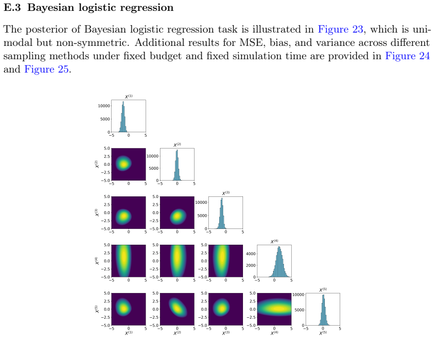
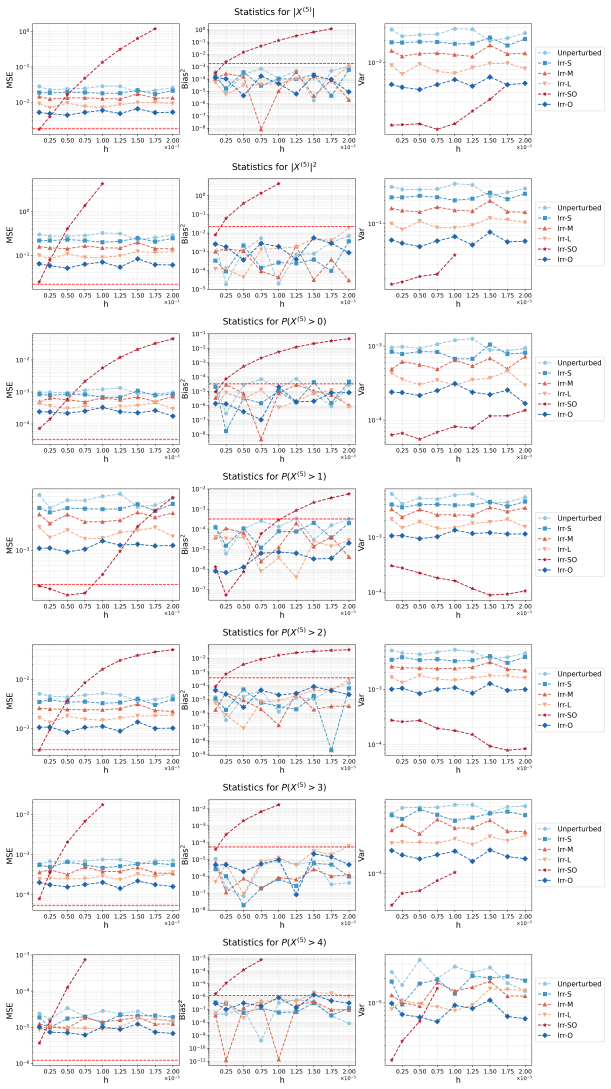
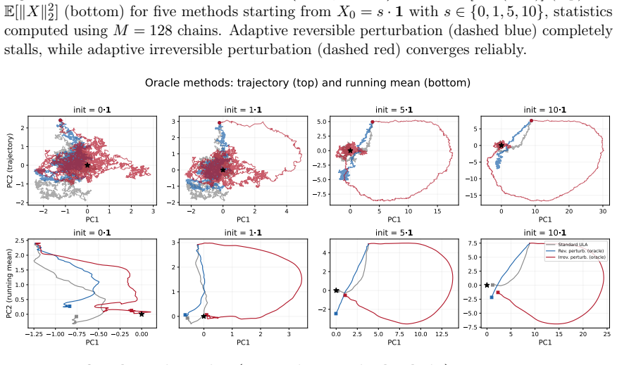
Optimizing Irreversible Perturbations of the Unadjusted Langevin Algorithm
Pith reviewed 2026-06-28 04:47 UTC · model grok-4.3
The pith
The paper derives an explicit characterization of the optimal position-independent irreversible perturbation for the unadjusted Langevin algorithm.
A machine-rendered reading of the paper's core claim, the machinery that carries it, and where it could break.
Core claim
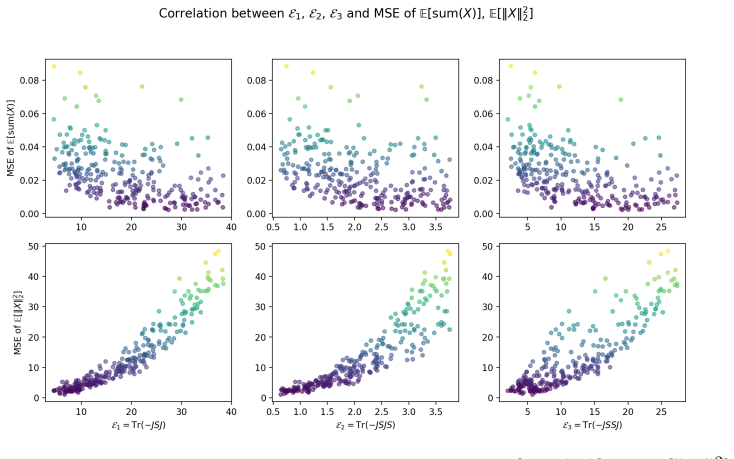
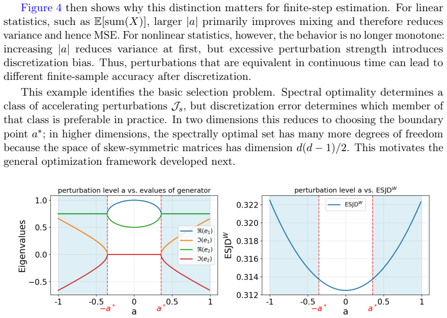
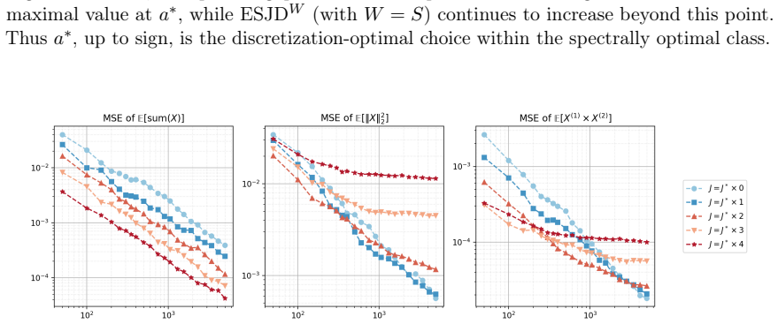
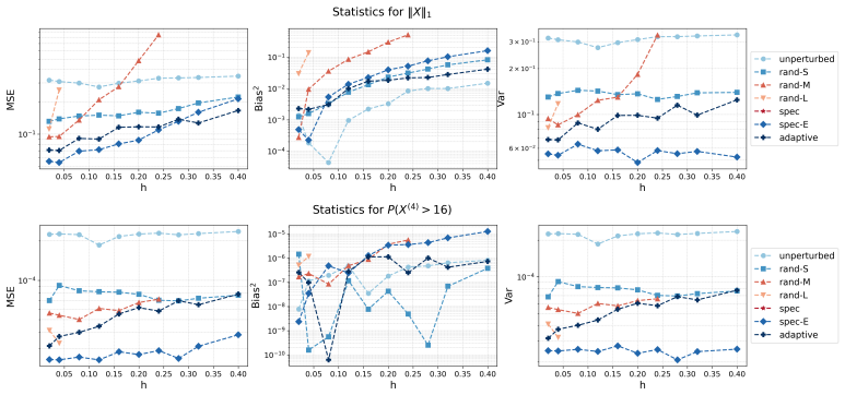
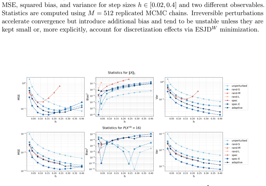
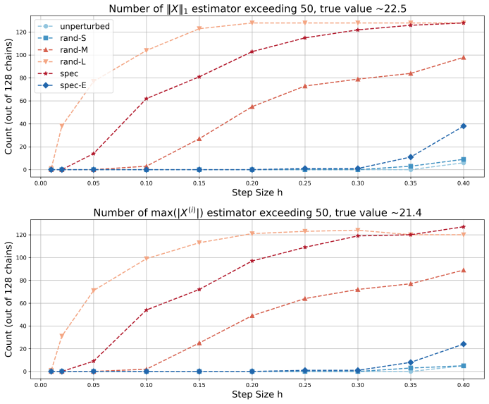
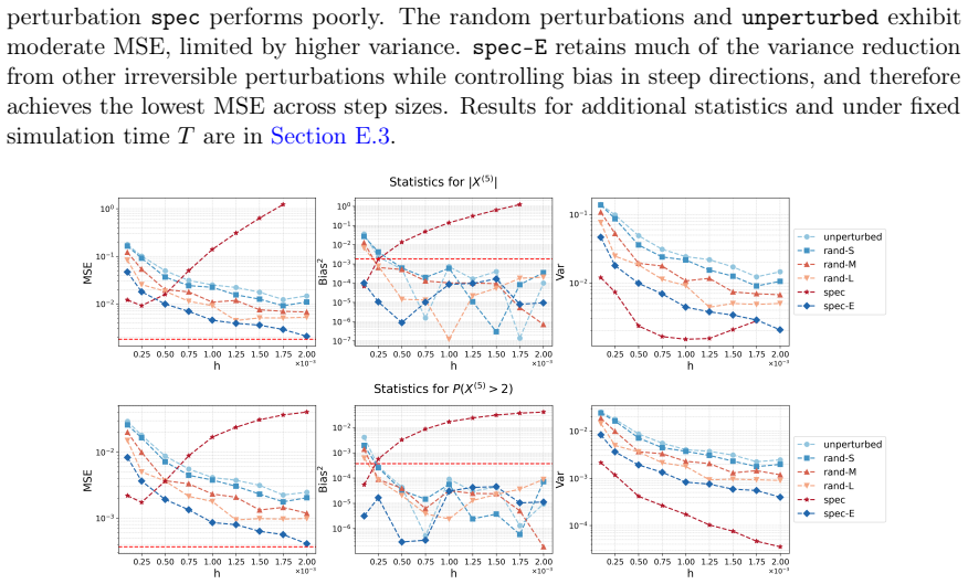
Within the proposed optimization framework, the optimal position-independent irreversible perturbation is explicitly characterized, leading to faster convergence with controlled bias in the unadjusted Langevin algorithm compared to other choices.
What carries the argument
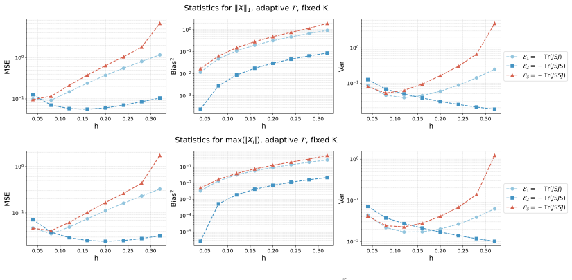
The constrained optimization problem that simultaneously maximizes a spectral gap analogue for mixing efficiency subject to a bound on the weighted expected squared jump distance for discretization bias.
If this is right
- The optimal perturbation is given by an explicit formula that does not require further numerical search.
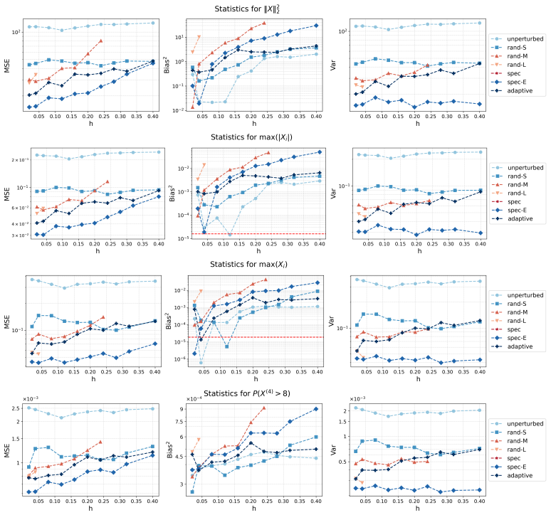
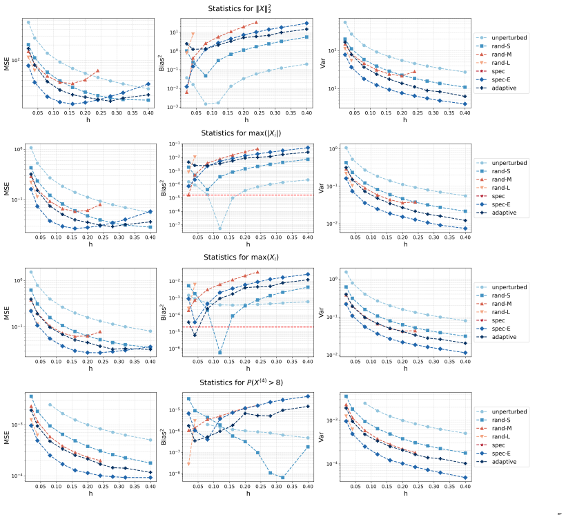
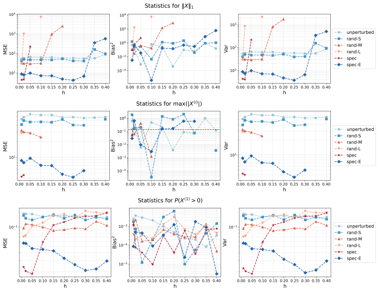
- Numerical experiments show faster convergence rates while maintaining controlled bias.
- Mean squared estimation errors are reduced compared to alternative irreversible perturbations.
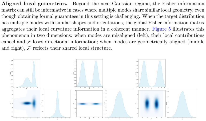
- The design improves performance for non-Gaussian target distributions where discretization effects are significant.
Where Pith is reading between the lines
- This framework may be extended to position-dependent perturbations for further gains.
- Similar joint optimization could apply to other Langevin-based samplers like the Metropolis-adjusted version.
- Testing on a wider range of high-dimensional distributions would reveal the practical scope of the explicit characterization.
- The modeling of bias via weighted jump distance suggests a general way to balance accuracy and speed in discrete MCMC methods.
Load-bearing premise
The assumption that mixing efficiency is captured by a spectral-gap analogue and discretization bias by a weighted expected squared jump distance.
What would settle it
An experiment showing that the explicitly derived optimal perturbation does not outperform standard choices in terms of convergence speed or estimation error on a given target distribution.
Figures


read the original abstract
Irreversible perturbations accelerate the convergence of Langevin dynamics, breaking detailed balance while preserving the invariant measure. The design of optimal irreversible perturbations has been studied in the continuous-time Gaussian setting, but extensions to non-Gaussian target distributions, and the impact of time discretization on the design of optimal perturbations, have not been well understood. Numerical discretizations of Langevin dynamics introduce bias, which is typically exacerbated by irreversible perturbations; handling this interaction demands a joint treatment of acceleration and accuracy. This paper develops a systematic framework for optimizing position-independent irreversible perturbations of the unadjusted Langevin algorithm (ULA). We formulate a constrained optimization problem that simultaneously accounts for mixing efficiency and discretization bias, where the former is characterized by a spectral gap analogue and the latter is quantified via a weighted expected squared jump distance. Within this framework, we derive an explicit characterization of the optimal position-independent irreversible perturbation. Extensive numerical experiments demonstrate that our design yields faster convergence with controlled bias, and improves mean squared estimation errors compared to other choices of irreversible perturbation.
Editorial analysis
A structured set of objections, weighed in public.
Referee Report
Summary. The paper develops a framework for optimizing position-independent irreversible perturbations of the unadjusted Langevin algorithm (ULA). It formulates a constrained optimization problem whose objective combines a spectral-gap analogue (for mixing efficiency) with a weighted expected squared jump distance (for discretization bias), derives an explicit characterization of the resulting optimal perturbation, and reports numerical experiments indicating faster convergence and lower mean-squared estimation error relative to other irreversible choices.
Significance. If the chosen proxies remain faithful outside the Gaussian setting and under discretization, the explicit characterization supplies a concrete, computable design rule that jointly controls acceleration and bias; this would extend prior continuous-time Gaussian results to practical non-Gaussian sampling and could be directly implemented in existing ULA codes.
major comments (2)
- [§3] §3 (Optimization framework): the spectral-gap analogue and weighted-ESJD objective are introduced as modeling choices without analytic bounds or numerical calibration showing that they preserve ranking of perturbations once the target leaves the Gaussian class or once step-size interacts with the irreversible drift; the explicit optimum is therefore guaranteed only inside the proxy model.
- [§4] §4 (Explicit characterization): the derivation of the closed-form perturbation relies on the stationarity and convexity properties asserted for the proxy objective; if those properties fail to hold for the true (non-Gaussian) generator, the claimed optimality does not transfer to the original mixing or bias metrics.
minor comments (2)
- Notation for the irreversible drift and the weighting function in the ESJD should be introduced with a single consistent symbol table.
- Figure captions should state the target distribution, step-size, and number of independent runs for each panel.
Simulated Author's Rebuttal
We thank the referee for the careful reading and the constructive major comments. We respond to each point below, acknowledging the modeling assumptions in our framework while defending the practical utility supported by our analysis and experiments. We will make partial revisions to clarify scope and limitations.
read point-by-point responses
-
Referee: [§3] §3 (Optimization framework): the spectral-gap analogue and weighted-ESJD objective are introduced as modeling choices without analytic bounds or numerical calibration showing that they preserve ranking of perturbations once the target leaves the Gaussian class or once step-size interacts with the irreversible drift; the explicit optimum is therefore guaranteed only inside the proxy model.
Authors: The proxies are deliberately introduced as tractable surrogates that extend known continuous-time Gaussian results to the discrete ULA setting while enabling an explicit solution. The paper does not claim analytic preservation of rankings for arbitrary non-Gaussian targets; instead, it motivates the choices via their correspondence to spectral properties and bias in the Gaussian case and then validates the resulting design through extensive numerical experiments on non-Gaussian targets (mixtures, heavy-tailed distributions) in Section 5. These experiments show consistent improvements in convergence and MSE. We will revise §3 to state the modeling assumptions more explicitly and to include a short additional calibration study on step-size interaction. revision: partial
-
Referee: [§4] §4 (Explicit characterization): the derivation of the closed-form perturbation relies on the stationarity and convexity properties asserted for the proxy objective; if those properties fail to hold for the true (non-Gaussian) generator, the claimed optimality does not transfer to the original mixing or bias metrics.
Authors: The closed-form result is derived and stated strictly for the proxy objective under the verified stationarity and convexity conditions within that model. The manuscript presents the design as a computable rule motivated by the proxy rather than a provably optimal perturbation for the true non-Gaussian generator. Numerical results on non-Gaussian examples support its effectiveness in practice. We will add a clarifying remark in §4 that emphasizes the proxy scope and notes that transfer to the original metrics is empirical. revision: partial
Circularity Check
No circularity: explicit characterization is the solution to the paper-defined constrained optimization problem
full rationale
The paper sets up its own objective (spectral-gap analogue for mixing + weighted ESJD for bias) and derives the perturbation that optimizes it within that framework. This is a standard optimization result, not a reduction of the claimed optimum to a fitted input or self-citation by construction. No load-bearing self-citations, no self-definitional loops, and no renaming of known results are indicated in the provided text. The derivation is self-contained against the proxies the authors explicitly adopt.
Axiom & Free-Parameter Ledger
Reference graph
Works this paper leans on
-
[1]
URL https://proceedings.neurips.cc/paper_files/paper/1995/file/ e19347e1c3ca0c0b97de5fb3b690855a-Paper.pdf
MIT Press. URL https://proceedings.neurips.cc/paper_files/paper/1995/file/ e19347e1c3ca0c0b97de5fb3b690855a-Paper.pdf. Christophe Andrieu, Nando De Freitas, Arnaud Doucet, and Michael I Jordan. An introduc- tion to mcmc for machine learning.Machine learning, 50(1):5–43,
1995
-
[2]
doi: 10.3150/18-BEJ1073. Brice Franke, C-R Hwang, H-M Pai, and S-J Sheu. The behavior of the spectral gap under growing drift.Transactions of the American Mathematical Society, 362(3):1325–1350,
-
[3]
URLhttps://arxiv.org/abs/1206.4665. Charles J Geyer. Practical markov chain monte carlo.Statistical science, pages 473–483,
-
[4]
doi: 10.1214/aoap/1177005371. Chii-Ruey Hwang, Shu-Yin Hwang-Ma, and Shuenn-Jyi Sheu. Accelerating diffusions.The Annals of Applied Probability, 15(2):1433–1444,
-
[5]
doi: 10.1214/105051605000000025. Frederick James. Monte carlo theory and practice.Reports on progress in Physics, 43(9): 1145–1189,
-
[6]
Tosio Kato.Perturbation theory for linear operators, volume
doi: 10.1088/0034-4885/43/9/002. Tosio Kato.Perturbation theory for linear operators, volume
-
[7]
ISSN 1572-9613. doi: 10.1007/s10955-013-0769-x. URL https://doi.org/10.1007/ s10955-013-0769-x. Jianfeng Lu and Konstantinos Spiliopoulos. Analysis of multiscale integrators for multiple attractors and irreversible langevin samplers.Multiscale Modeling & Simulation, 16(4): 1859–1883,
-
[8]
Fisher discriminant analysis with kernels
Sebastian Mika, Gunnar Rätsch, Jason Weston, Bernhard Schölkopf, and Klaus-Robert Müller. Fisher discriminant analysis with kernels. InProceedings of the 1999 IEEE Signal Processing Society Workshop on Neural Networks for Signal Processing IX, pages 41–48. IEEE,
1999
-
[9]
doi: 10.1109/NNSP.1999.788121. 58 Antonietta Mira. Ordering and improving the performance of monte carlo markov chains. Statistical Science, pages 340–350,
-
[10]
Improving Asymptotic Variance of MCMC Estimators: Non-reversible Chains are Better
doi: 10.1090/fic/026/07. Radford M Neal. Improving asymptotic variance of mcmc estimators: Non-reversible chains are better.arXiv preprint math/0407281,
work page internal anchor Pith review Pith/arXiv arXiv doi:10.1090/fic/026/07
-
[11]
Matthew D Parno and Youssef M Marzouk
doi: 10.1007/s40072-019-00147-5. Matthew D Parno and Youssef M Marzouk. Transport map accelerated markov chain monte carlo.SIAM/ASA Journal on Uncertainty Quantification, 6(2):645–682,
-
[12]
https://link.springer.com/book/10.1007/978-1-4939-1323-7
doi: 10.1007/978-1-4939-1323-7. Michael Reed and Barry Simon.Methods of Modern Mathematical Physics II: Fourier Analysis, Self-Adjointness, volume
-
[13]
Luc Rey-Bellet and Konstantinos Spiliopoulos. Irreversible langevin samplers and variance reduction: a large deviations approach.Nonlinearity, 28(7):2081–2103, May 2015a. ISSN 1361-6544. doi: 10.1088/0951-7715/28/7/2081. Luc Rey-Bellet and Konstantinos Spiliopoulos. Variance reduction for irreversible langevin samplers and diffusion on graphs.Electronic C...
-
[14]
doi: 10.1007/s10955-016-1565-1. Christian P. Robert and George Casella.Monte Carlo Statistical Methods. Springer Texts in Statistics. Springer, New York,
-
[15]
Gareth O Roberts and Jeffrey S Rosenthal
doi: 10.1007/978-1-4757-3071-5. Gareth O Roberts and Jeffrey S Rosenthal. Optimal scaling of discrete approximations to langevin diffusions.Journal of the Royal Statistical Society: Series B (Statistical Methodology), 60(1):255–268,
-
[16]
Max Welling and Yee Teh
URLhttps://proceedings.neurips.cc/paper_files/ paper/2023/file/5da6d5818a156791090c875abeca3cf8-Paper-Conference.pdf. Max Welling and Yee Teh. Bayesian learning via stochastic gradient langevin dynamics. In Proceedings of the 28th International Conference on Machine Learning (ICML), pages 681–688. Omnipress, 01
2023
discussion (0)
Sign in with ORCID, Apple, or X to comment. Anyone can read and Pith papers without signing in.