Percolation and clustering in ecological communities: A dynamical theory
Pith reviewed 2026-06-27 14:11 UTC · model grok-4.3
The pith
Dynamical accessibility of equilibria in a discrete Lotka-Volterra model determines the onset of percolation and clustering on random interaction graphs.
A machine-rendered reading of the paper's core claim, the machinery that carries it, and where it could break.
Core claim
Within the discrete generalized Lotka-Volterra framework on random graphs, the set of equilibria that the dynamics can actually reach governs the emergence of percolating clusters and the spatial organization of surviving sites, so that dynamical accessibility, rather than the mere existence of equilibria, sets the thresholds for clustering and percolation.
What carries the argument
The discrete generalized Lotka-Volterra model on random interaction graphs, whose reachable equilibria dictate the onset of percolation and clustering.
If this is right
- Percolation occurs only when the dynamics can reach equilibria that support a giant connected component of surviving sites.
- The spatial patterns of surviving species are fixed by the subset of equilibria the dynamics can attain.
- Clustering thresholds are set by the boundary between reachable and unreachable equilibria rather than by static stability alone.
- The discrete formulation yields explicit analytical conditions for the transition to percolating states.
Where Pith is reading between the lines
- The same reachability constraint may limit collective organization in continuous-time versions or in graphs with different degree distributions.
- Controlled perturbations that block specific equilibria could be used to test whether percolation disappears as predicted.
- The approach suggests a general route for analyzing dynamical selection of phases in other network-based population models.
Load-bearing premise
The discrete version of the generalized Lotka-Volterra model preserves the key macroscopic features of continuous ecological dynamics.
What would settle it
A concrete counter-example would be a realized random graph where the dynamics reach only non-percolating equilibria yet percolation is nevertheless observed in the steady state, or where an accessible equilibrium predicts percolation but none appears.
Figures
read the original abstract
Ecological communities with structured interactions exhibit collective phenomena such as percolation and clustering of occupied sites. While these effects have been documented in experiments and simulations, systematic analytical understanding has remained limited. In this paper, we develop a dynamical theory of these phenomena for competitive ecological systems defined on random interaction graphs. We introduce a discrete version of the generalized Lotka-Volterra model that preserves key macroscopic features of continuous ecological dynamics while enabling analytical treatment. Within this framework, we characterize the emergence of percolating clusters and describe the spatial organization of surviving sites. Our analysis uncovers which equilibria can be reached by the dynamics and shows how this dynamical accessibility governs the onset of clustering and percolation. In doing so, our framework complements classical Lotka-Volterra theory by providing a dynamical perspective on the collective organization of structured communities.
Editorial analysis
A structured set of objections, weighed in public.
Referee Report
Summary. The paper develops a dynamical theory of percolation and clustering for competitive ecological communities on random interaction graphs. It introduces a discrete generalized Lotka-Volterra model asserted to preserve key macroscopic features of the continuous dynamics, enabling analytical characterization of reachable equilibria; the central claim is that dynamical accessibility of these equilibria governs the onset and spatial organization of clustering and percolation, thereby complementing classical Lotka-Volterra theory.
Significance. If the modeling choice and equilibrium analysis hold, the work supplies an analytical link between dynamical reachability and collective network phenomena that have previously been studied mainly via simulation or experiment. This could furnish falsifiable predictions for structured communities and a reproducible discrete framework for further theoretical exploration.
minor comments (2)
- [Abstract] The abstract states that the discrete model 'preserves key macroscopic features' but does not indicate where in the manuscript a direct comparison (e.g., steady-state distributions or invasion criteria) with the continuous GLV is provided; adding a short explicit statement or reference to the relevant section would strengthen the claim.
- [Methods] Notation for the random interaction graph and the discrete update rule should be introduced with a single consolidated table or figure early in the methods to avoid repeated re-definition later.
Simulated Author's Rebuttal
We thank the referee for their positive summary of the work, recognition of its potential significance, and recommendation for minor revision. No specific major comments were raised in the report.
Circularity Check
No significant circularity; derivation self-contained
full rationale
The abstract presents the discrete GLV variant as an explicit modeling choice chosen to preserve macroscopic features while enabling analysis, with subsequent claims about reachable equilibria, clustering, and percolation framed as results of that analysis. No equations, fitted parameters, self-citations, or ansatzes are quoted that reduce any prediction or uniqueness claim back to the inputs by construction. The load-bearing step (preservation of macroscopic features) is stated as an assumption rather than derived, leaving the framework independent of the target results.
Axiom & Free-Parameter Ledger
Reference graph
Works this paper leans on
-
[1]
Rietkerk and J
M. Rietkerk and J. van de Koppel, Regular pattern for- mation in real ecosystems, Trends Ecol. Evol.23, 169 (2008)
2008
-
[2]
Borgogno, P
F. Borgogno, P. D’Odorico, F. Laio, and L. Ridolfi, Mathematical models of vegetation pattern formation in ecohydrology, Reviews of Geophysics47(2009)
2009
-
[3]
Manor and N
A. Manor and N. M. Shnerb, Facilitation, competition, and vegetation patchiness: from scale free distribution to patterns, J. Theor. Biol.253, 838 (2008)
2008
-
[4]
Dakos, S
V. Dakos, S. K´ efi, M. Rietkerk, E. H. van Nes, and M. Scheffer, Slowing down in spatially patterned ecosys- tems at the brink of collapse., The American Naturalist 177, E153 (2011), pMID: 21597246
2011
-
[5]
K´ efi, M
S. K´ efi, M. Rietkerk, C. L. Alados, Y. Pueyo, V. P. Pa- panastasis, A. Elaich, and P. C. de Ruiter, Spatial vege- tation patterns and imminent desertification in mediter- ranean arid ecosystems, Nature449, 213 (2007)
2007
-
[6]
von Hardenberg, E
J. von Hardenberg, E. Meron, M. Shachak, and Y. Zarmi, Diversity of vegetation patterns and deser- tification, Phys. Rev. Lett.87, 198101 (2001)
2001
-
[7]
Rietkerk, M
M. Rietkerk, M. C. Boerlijst, F. van Langevelde, R. Hil- lerislambers, J. van de Koppel, L. Kumar, H. H. T. Prins, and A. M. de Roos, Self-organization of vegeta- tion in arid ecosystems, Am. Nat.160, 524 (2002)
2002
-
[8]
Hogeweg, Cellular automata as a paradigm for eco- logical modeling, Appl
P. Hogeweg, Cellular automata as a paradigm for eco- logical modeling, Appl. Math. Comput.27, 81 (1988)
1988
-
[9]
G. B. Ermentrout and L. Edelstein-Keshet, Cellular au- tomata approaches to biological modeling, J. Theor. Biol.160, 97 (1993)
1993
-
[10]
Deutsch and S
A. Deutsch and S. Dormann,Cellular automaton modeling of biological pattern formation, Modeling and Simulation in Science, Engineering & Technology (Birkh¨ auser Boston, Boston, MA, 2017)
2017
-
[11]
A. M. Turing, The chemical basis of morphogenesis. 1953, Bull. Math. Biol.52, 153 (1990)
1953
-
[12]
D’Odorico, F
P. D’Odorico, F. Laio, and L. Ridolfi, Patterns as indi- cators of productivity enhancement by facilitation and competition in dryland vegetation, J. Geophys. Res. 111(2006)
2006
-
[13]
Lejeune, P
O. Lejeune, P. Couteron, and R. Lefever, Short range co-operativity competing with long range inhibition ex- plains vegetation patterns, Acta Oecol. (Montrouge) 20, 171 (1999)
1999
-
[14]
K´ efi, V
S. K´ efi, V. Guttal, W. A. Brock, S. R. Carpenter, A. M. Ellison, V. N. Livina, D. A. Seekell, M. Scheffer, E. H. van Nes, and V. Dakos, Early warning signals of eco- logical transitions: methods for spatial patterns, PLoS One9, e92097 (2014)
2014
-
[15]
Vega and C
E. Vega and C. Monta˜ na, Effects of overgrazing and rainfall variability on the dynamics of semiarid banded vegetation patterns: A simulation study with cellular automata, Journal of Arid Environments75, 70 (2011)
2011
-
[16]
Ge, The hidden order of turing patterns in arid and semi-arid vegetation ecosystems, Proceedings of the Na- tional Academy of Sciences120, e2306514120 (2023)
Z. Ge, The hidden order of turing patterns in arid and semi-arid vegetation ecosystems, Proceedings of the Na- tional Academy of Sciences120, e2306514120 (2023)
2023
-
[17]
Volterra, Fluctuations in the abundance of a species considered mathematically, Nature118, 558–560 (1926)
V. Volterra, Fluctuations in the abundance of a species considered mathematically, Nature118, 558–560 (1926)
1926
-
[18]
Volterra, Fluctuations dans la lutte pour la vie, leurs lois fondamentales et de r´ eciprocit´ e, Bull
V. Volterra, Fluctuations dans la lutte pour la vie, leurs lois fondamentales et de r´ eciprocit´ e, Bull. Soc. Math. France (1939)
1939
-
[19]
Grilli, T
J. Grilli, T. Rogers, and S. Allesina, Modularity and stability in ecological communities, Nat. Commun.7, 12031 (2016)
2016
-
[20]
K. Z. Coyte, J. Schluter, and K. R. Foster, The ecology of the microbiome: Networks, competition, and stabil- ity, Science350, 663 (2015)
2015
-
[21]
Faust and J
K. Faust and J. Raes, Microbial interactions: from net- works to models, Nat. Rev. Microbiol.10, 538 (2012)
2012
-
[22]
MacArthur, Species packing and competitive equilib- rium for many species, Theor
R. MacArthur, Species packing and competitive equilib- rium for many species, Theor. Popul. Biol.1, 1 (1970)
1970
-
[23]
Biroli, G
G. Biroli, G. Bunin, and C. Cammarota, Marginally stable equilibria in critical ecosystems, New Journal of Physics20, 083051 (2018)
2018
-
[24]
A. Altieri, F. Roy, C. Cammarota, and G. Biroli, Prop- erties of equilibria and glassy phases of the random lotka-volterra model with demographic noise, Physical Review Letters126, 10.1103/physrevlett.126.258301 (2021)
-
[25]
Bunin, Ecological communities with lotka-volterra dynamics, Phys
G. Bunin, Ecological communities with lotka-volterra dynamics, Phys. Rev. E95, 042414 (2017)
2017
-
[26]
Marcus, A
S. Marcus, A. M. Turner, and G. Bunin, Local and collective transitions in sparsely-interacting ecological communities, PLoS Comput. Biol.18, e1010274 (2022)
2022
-
[27]
Tonolo, M
T. Tonolo, M. C. Angelini, S. Azaele, A. Maritan, and G. Gradenigo, Generalized Lotka-Volterra model with sparse interactions: Non-Gaussian effects and topolog- ical multiple-equilibria phase, PRX Life4(2026)
2026
-
[28]
V. Ros, F. Roy, G. Biroli, G. Bunin, and A. M. Turner, Generalized lotka-volterra equations with random, non- reciprocal interactions: The typical number of equilib- ria, Phys. Rev. Lett.130, 257401 (2023)
2023
-
[29]
Chesson, MacArthur’s consumer-resource model, Theor
P. Chesson, MacArthur’s consumer-resource model, Theor. Popul. Biol.37, 26 (1990)
1990
-
[30]
L. Fant, I. Macocco, and J. Grilli, Eco-evolutionary dy- namics lead to functionally robust and redundant com- munities (2021)
2021
-
[31]
J. Gore, J. Hu, Y. He, M. Barbier, J. Song, and G. Bunin, Transition from global stability to multiple attractors in microcosms (2025)
2025
-
[32]
Aguirre-L´ opez, Heterogeneous mean-field analysis of the generalized Lotka–Volterra model on a network, J
F. Aguirre-L´ opez, Heterogeneous mean-field analysis of the generalized Lotka–Volterra model on a network, J. Phys. A Math. Theor.57, 345002 (2024)
2024
-
[33]
Advani, G
M. Advani, G. Bunin, and P. Mehta, Statistical physics of community ecology: a cavity solution to macarthur’s consumer resource model, Journal of Statistical Me- chanics: Theory and Experiment2018, 033406 (2018)
2018
-
[34]
W. Cui, R. Marsland, and P. Mehta, Effect of re- source dynamics on species packing in diverse ecosys- tems, Physical Review Letters125, 10.1103/phys- revlett.125.048101 (2020)
-
[35]
B. R. Silliman, M. J. Hensel, J. P. Gibert, P. Daleo, C. S. Smith, D. J. Wieczynski, C. Angelini, A. B. Pax- ton, A. M. Adler, Y. S. Zhang, A. H. Altieri, T. M. Palmer, H. P. Jones, R. K. Gittman, J. N. Griffin, M. I. O’Connor, J. van de Koppel, J. R. Poulsen, M. Rietk- erk, Q. He, M. D. Bertness, T. van der Heide, and S. R. Valdez, Harnessing ecological ...
2024
-
[36]
R. J. Orth, J. S. Lefcheck, K. S. McGlathery, L. Aoki, M. W. Luckenbach, K. A. Moore, M. P. J. Oreska, R. Snyder, D. J. Wilcox, and B. Lusk, Restoration 11 of seagrass habitat leads to rapid recovery of coastal ecosystem services, Science Advances6, eabc6434 (2020)
2020
-
[37]
A. J. Wells, J. Harrington, and N. J. Balster, Seeding density alters the assembly of a restored plant commu- nity after the removal of a dam in southern wisconsin, usa, Environments11, 10.3390/environments11060115 (2024)
-
[38]
J. D. Corbin and K. D. Holl, Applied nucleation as a forest restoration strategy, Forest Ecology and Manage- ment265, 37 (2012)
2012
-
[39]
M. L. E. Gr¨ afnings, J. H. T. Heusinkveld, N. Hijner, D. J. J. Hoeijmakers, Q. Smeele, M. Zwarts, T. van der Heide, and L. L. Govers, Spatial design improves effi- ciency and scalability of seed-based seagrass restoration, Journal of Applied Ecology60, 967 (2023)
2023
-
[40]
E. L. Kjaer, G. R. Houseman, K. N. Luu, B. L. Foster, L. Laanisto, and A. J. Golubski, Spatial pattern of seed arrival has a greater effect on plant diversity than does soil heterogeneity in a grassland ecosystem, Plant Soil (2024)
2024
-
[41]
Behrens, B
F. Behrens, B. Hudcov´ a, and L. Zdeborov´ a, Backtrack- ing dynamical cavity method, Phys. Rev. X13, 031021 (2023)
2023
-
[42]
Behrens, B
F. Behrens, B. Hudcov´ a, and L. Zdeborov´ a, Dynamical phase transitions in graph cellular automata, Phys. Rev. E109, 044312 (2024)
2024
-
[43]
H. Sun, S. Chen, J. Xie, and Y. Hu, Growth-induced percolation on complex networks, PNAS Nexus4, pgaf192 (2025)
2025
-
[44]
Timonin, Statistics of geometric clusters in the ising model on a bethe lattice, Physica A: Statistical Mechan- ics and its Applications527, 121402 (2019)
P. Timonin, Statistics of geometric clusters in the ising model on a bethe lattice, Physica A: Statistical Mechan- ics and its Applications527, 121402 (2019)
2019
-
[45]
D. S. Callaway, M. E. J. Newman, S. H. Strogatz, and D. J. Watts, Network robustness and fragility: Perco- lation on random graphs, Phys. Rev. Lett.85, 5468 (2000)
2000
-
[46]
Karrer and M
B. Karrer and M. E. J. Newman, Message passing ap- proach for general epidemic models, Phys. Rev. E82, 016101 (2010)
2010
-
[47]
Karrer, M
B. Karrer, M. E. J. Newman, and L. Zdeborov´ a, Perco- lation on sparse networks, Phys. Rev. Lett.113, 208702 (2014)
2014
-
[48]
M. E. J. Newman, Spread of epidemic disease on net- works, Phys. Rev. E66, 016128 (2002)
2002
-
[49]
Cohen, K
R. Cohen, K. Erez, D. ben Avraham, and S. Havlin, Resilience of the internet to random breakdowns, Phys. Rev. Lett.85, 4626 (2000)
2000
-
[50]
J. Xie, X. Wang, L. Feng, J.-H. Zhao, W. Liu, Y. Moreno, and Y. Hu, Indirect influence in social networks as an induced percolation phenomenon, Pro- ceedings of the National Academy of Sciences119, e2100151119 (2022)
2022
-
[51]
Shrestha, S
M. Shrestha, S. V. Scarpino, and C. Moore, Message- passing approach for recurrent-state epidemic models on networks, Phys. Rev. E92, 022821 (2015)
2015
-
[52]
Dobrinevski and E
A. Dobrinevski and E. Frey, Extinction in neutrally sta- ble stochastic lotka-volterra models, Phys. Rev. E85, 051903 (2012)
2012
-
[53]
J. Knebel, M. F. Weber, T. Kr¨ uger, and E. Frey, Evolutionary games of condensates in coupled birth–death processes, Nature Communications6, 10.1038/ncomms7977 (2015)
-
[54]
M. M. Desai and D. S. Fisher, Beneficial muta- tion–selection balance and the effect of linkage on pos- itive selection, Genetics176, 1759 (2007)
2007
-
[55]
Stauffer and A
D. Stauffer and A. Aharony,Introduction to percolation theory, 2nd ed. (Taylor & Francis, Philadelphia, PA, 1992)
1992
-
[56]
Erd˝ os and A
P. Erd˝ os and A. R´ enyi, On the evolution of random graphs, Publ. Math. Inst. Hung. Acad. Sci. (1960)
1960
-
[57]
C. A. Klausmeier, Regular and irregular patterns in semiarid vegetation, Science284, 1826–1828 (1999)
1999
-
[58]
M´ ezard and A
M. M´ ezard and A. Montanari,Information, Physics, and Computation(2009)
2009
-
[59]
M. E. J. Newman, Threshold effects for two pathogens spreading on a network, Phys. Rev. Lett.95, 108701 (2005)
2005
-
[60]
V. Ros, F. Roy, G. Biroli, and G. Bunin, Quenched complexity of equilibria for asymmetric generalized lotka–volterra equations, Journal of Physics A: Mathe- matical and Theoretical56, 305003 (2023)
2023
-
[61]
Jankola, F
M. Jankola, F. Behrens, C. Koller, and L. Zdeborov´ a, Minority takeover in majority dynamics: Searching for rare initializations via the history passing algorithm, Phys. Rev. E113, 064303 (2026)
2026
-
[62]
Koller, F
C. Koller, F. Behrens, and L. Zdeborov´ a, Counting and hardness-of-finding fixed points in cellular automata on random graphs, J. Phys. A Math. Theor.57, 465001 (2024)
2024
-
[63]
Zdeborov´ a and F
L. Zdeborov´ a and F. Krzakala, Statistical physics of in- ference: thresholds and algorithms, Advances in Physics 65, 453 (2016)
2016
-
[64]
M. E. J. Newman, S. H. Strogatz, and D. J. Watts, Random graphs with arbitrary degree distributions and their applications, Phys. Rev. E64, 026118 (2001)
2001
-
[65]
Paszke, S
A. Paszke, S. Gross, F. Massa, A. Lerer, J. Brad- bury, G. Chanan, T. Killeen, Z. Lin, N. Gimelshein, L. Antiga, A. Desmaison, A. K¨ opf, E. Z. Yang, Z. De- Vito, M. Raison, A. Tejani, S. Chilamkurthy, B. Steiner, L. Fang, J. Bai, and S. Chintala, Pytorch: An imper- ative style, high-performance deep learning library., in NeurIPS(2019) pp. 8024–8035. 12 A...
2019
-
[66]
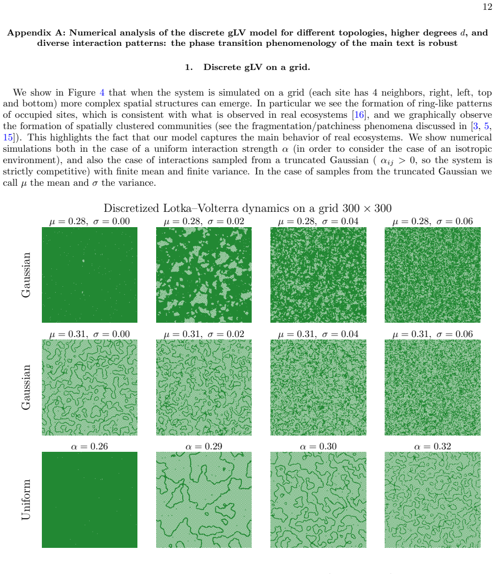
We show in Figure 4 that when the system is simulated on a grid (each site has 4 neighbors, right, left, top and bottom) more complex spatial structures can emerge
Discrete gLV on a grid. We show in Figure 4 that when the system is simulated on a grid (each site has 4 neighbors, right, left, top and bottom) more complex spatial structures can emerge. In particular we see the formation of ring-like patterns of occupied sites, which is consistent with what is observed in real ecosystems [16], and we graphically observ...
-
[67]
normalized
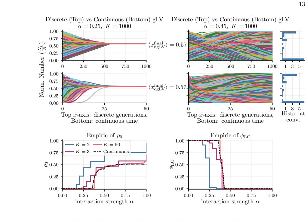
The discrete dynamic in the limit of largeK. We show that for largeKthe discrete gLV model in Eq. (2) approximates very well the continuous model in Eq. (1). We carry out numerical integration of the differential equations for continuous dynamical rule in Eq. (1) 13 0 250 500 750 1000 0.00 0.25 0.50 0.75 1.00 Discrete (Top) vs Continuous (Bottom) gL V α= ...
-
[68]
We simulate our dynamics for heterogeneous interaction strengths and measure the observablesρ 0 andϕ LC, the results are shown in Figure 6
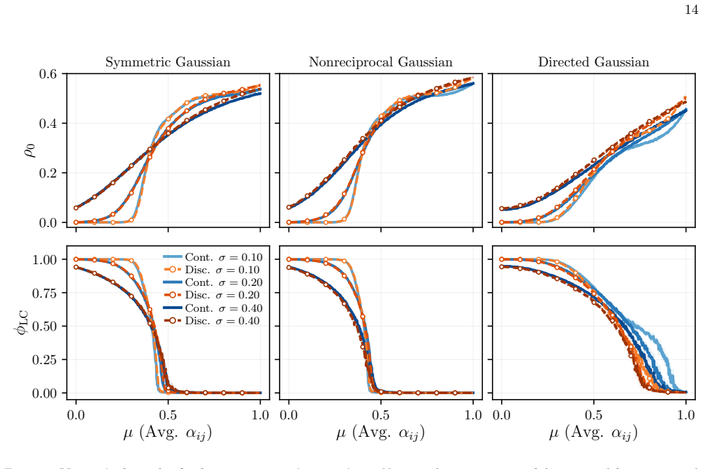
Numerical simulations on tree-like graphs with non-uniform interactions. We simulate our dynamics for heterogeneous interaction strengths and measure the observablesρ 0 andϕ LC, the results are shown in Figure 6. In particular, we consider the following distributions for the couplingsα ij. For the discrete model we fix the carrying capacity toK= 100, and ...
-
[69]
Symmetric Gaussian.α ij sampled from a truncated Gaussian distribution with the constraintα ij =α ji (symmetric interactions). We consider distinct values of the varianceσ, while we callµthe average interaction strength 14 0.0 0.2 0.4 0.6 ρ0 Symmetric Gaussian Nonreciprocal Gaussian Directed Gaussian 0.0 0.5 1.0 µ (Avg. αij) 0.00 0.25 0.50 0.75 1.00 φLC C...
-
[70]
Nonreciprocal Gaussian.α ij sampled from a truncated Gaussian distribution without any symmetry con- straint (asymmetric interactions)
-
[71]
converge
Directed Gaussian.α ij sampled from a truncated Gaussian distribution with the constraint that ifα ij >0 thenα ji = 0, corresponding to a directed network (i.e., interactions are one-way). For comparison, we also simulate the continuous gLV model on systems of the same size. We find that the behavior ofρ 0 andϕ LC is qualitatively similar across all sampl...
-
[72]
variational
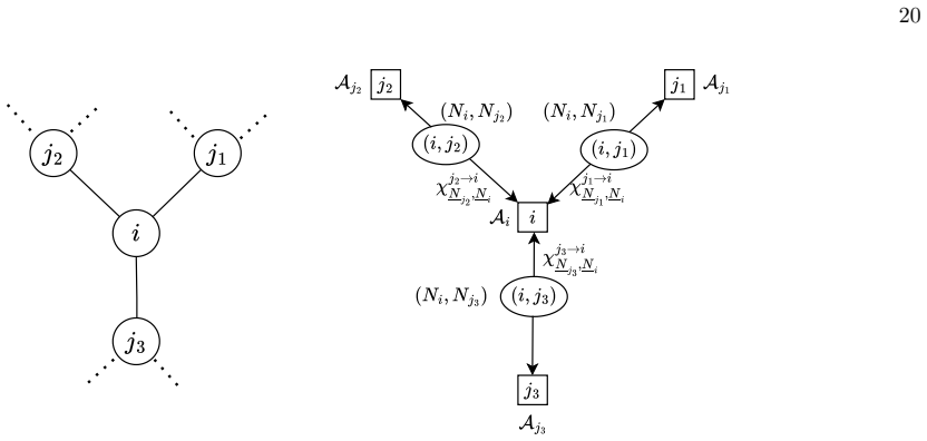
The Backtracking Dynamical Cavity Method Detailed expressions of the probability distributions needed to computeαatyp,α ext and observables. We now detail how to compute the entropy Φ (p/c) and the average values of the observables with respect to the following two probability distributions, adopting the same procedure originally introduced in [41, 42]. F...
-
[73]
X h∈∂i\j αihN t h X h∈∂i\j αihN t′ h # −E {N h∼ψh}h∈∂i\j
High degree limit of the BDCM equations Derivation of the expression of the messages in the high degree limit.We derive now the high degree limit of the BDCM equations. For generality, let’s considerα ij to be i.i.d. with varianceσ/ √ dand expectation α/d, for ad-regular graph. The goal is to take the limitd→ ∞, and we will later focus on the caseσ= 0 (un...
-
[74]
Message passing for dynamics-dependent percolation In this section, we develop the general message passing approach that we use to study the percolation of an attractor of the gLV dynamic. We stress from the start that the equations derived below can be applied to any dynamical system, including stochastic ones, whose underlying probability measure admits...
-
[75]
Simplifying the general percolation recursion with an approximation.The approach we developed in the previous section is asymptotically exact, but solving the recursion in Eq
(one can do exactly the same argument for bond percolation and find the recursion reported in [47]). Simplifying the general percolation recursion with an approximation.The approach we developed in the previous section is asymptotically exact, but solving the recursion in Eq. (D46) may still be complicated. Thus, we introduce an approximation that signifi...
-
[76]
˜η (i) l (N p+1 i ,{N p+1 j }j∈∂i) is an indicator function that equals 1 if siteiis occupied and connected toloccupied neighbors, and 0 otherwise
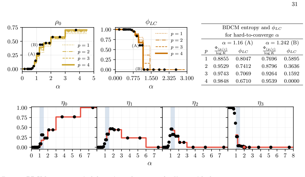
Computing the structure functionsη(ℓ)with FFT To compute this observable, we introduce the following edge localized observable ˜ηl(Np+1) = 1 S SX i=1 1[N p+1 i >0]1 hX j∈∂i 1[N p+1 j >0] =l i = 1 S SX i ˜η(i) l (N p+1 i ,{N p+1 j }j∈∂i).(E2) Remember that if a site is occupied at timep+ 1 it will be occupied over the full attractor. ˜η (i) l (N p+1 i ,{N ...
-
[77]
smallest possible initialization
General properties about the percolation fixed point recursion and discussion about the initialization We start by firstly defining the shorthandq iℓ→i N iℓ ,N i =H iℓ→i N iℓ ,N i (1) and to write the percolation recursion in Eq. (D47), specialized to the BDCM case, as qiℓ→i N iℓ ,N i = 1,ifA iℓ = 0, P {N u}u∈∂iℓ \i Aiℓ N iℓ , N i,{N u}u∈∂iℓ\i Q...
-
[78]
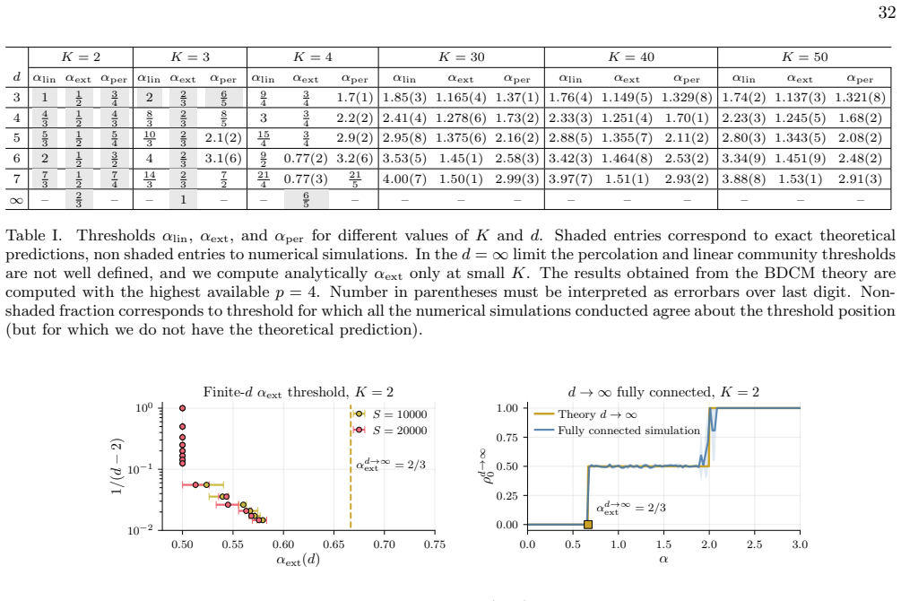
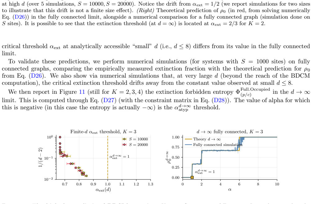
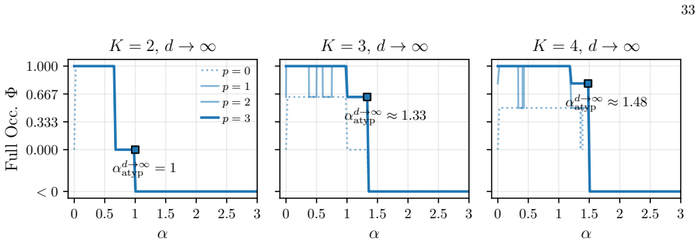
(D24), which allow us to compute the extinction fractionρ 0 (via Eq
Computing the critical extinction threshold and the atypical threshold atd=∞ We present in Figure 9 (K= 2) and Figure 10 (K= 3) the numerical solutions of Eq. (D24), which allow us to compute the extinction fractionρ 0 (via Eq. (D26)) in the fully connected limit (d=∞), and thus determine the corresponding extinction thresholdα d→∞ ext . These results sup...
-
[79]
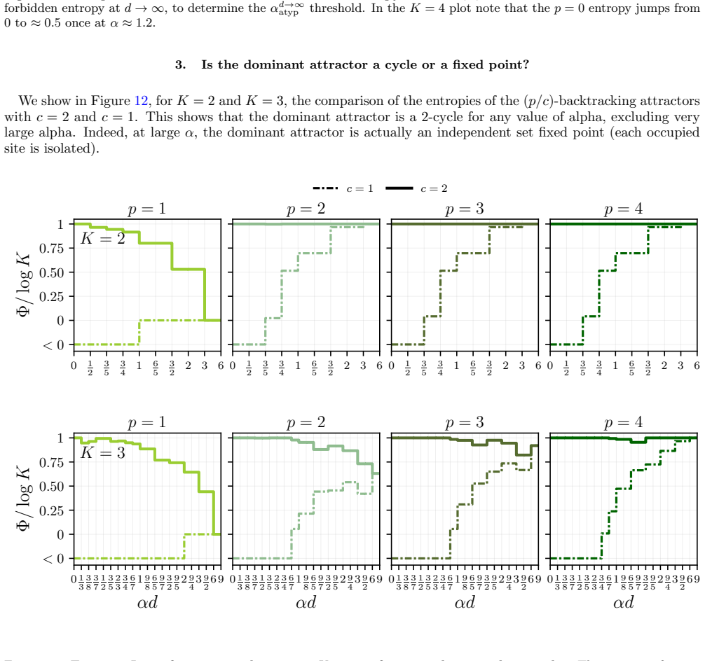
This shows that the dominant attractor is a 2-cycle for any value of alpha, excluding very large alpha
Is the dominant attractor a cycle or a fixed point? We show in Figure 12, forK= 2 andK= 3, the comparison of the entropies of the (p/c)-backtracking attractors withc= 2 andc= 1. This shows that the dominant attractor is a 2-cycle for any value of alpha, excluding very large alpha. Indeed, at largeα, the dominant attractor is actually an independent set fi...
-
[80]
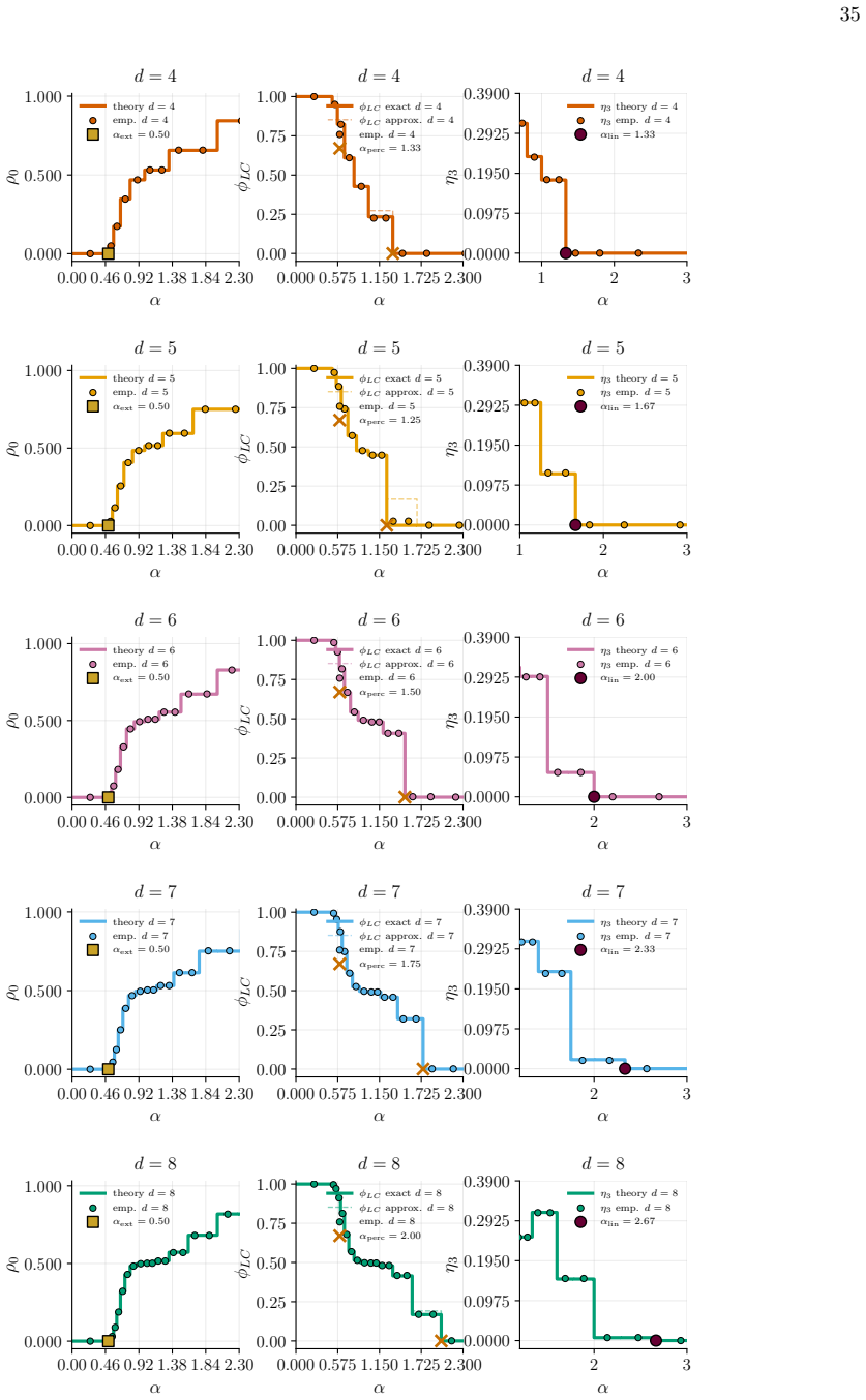
We show also the value ofϕ LC obtained with the approximation discussed in Appendix D 3, and compare it with the exact result
Additional plots forK= 2andd≥3 We show in Figure 13 the comparison between numerical simulations and theory for higherd. We show also the value ofϕ LC obtained with the approximation discussed in Appendix D 3, and compare it with the exact result. This supports the claim that the approximation works very well for almost alld, as the differences between ap...
1950
discussion (0)
Sign in with ORCID, Apple, or X to comment. Anyone can read and Pith papers without signing in.