Continuous biome representations from Earth observation embeddings
Pith reviewed 2026-06-27 10:21 UTC · model grok-4.3
The pith
A linear classifier on satellite embeddings turns categorical biome maps into continuous probability vectors that improve species occurrence prediction.
A machine-rendered reading of the paper's core claim, the machinery that carries it, and where it could break.
Core claim
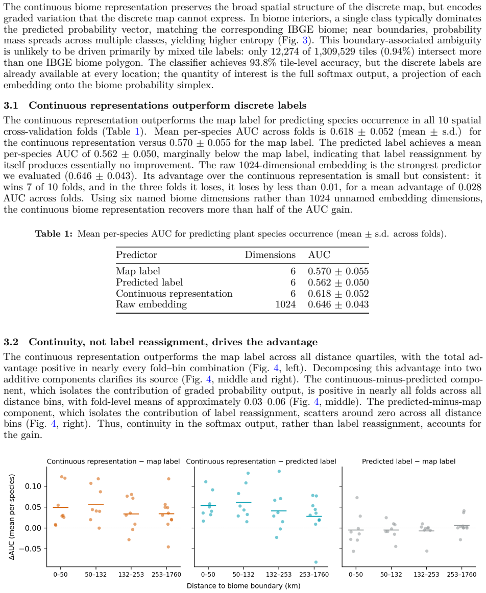
Training a linear classifier on Clay v1.5 satellite image embeddings to predict biome labels and taking the softmax as a continuous probability vector over biome classes produces representations that outperform discrete biome labels when predicting species occurrence, with mean per-species AUC rising from 0.570 to 0.618 across 10 spatial cross-validation folds on 10,015 withheld plots. The improvement is attributable to continuity in the graded output rather than label reassignment and holds at all distances from biome boundaries; the raw 1024-dimensional embedding reaches 0.646 but the continuous vector recovers most of that advantage.
What carries the argument
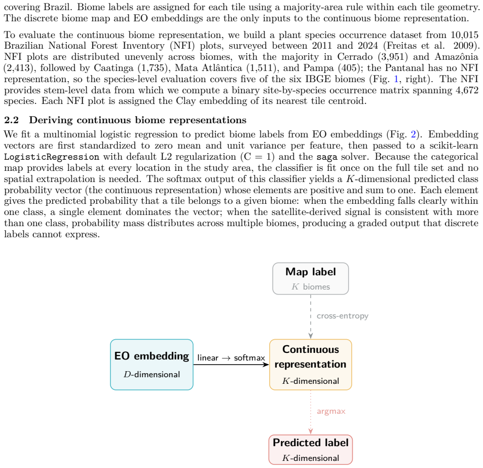
The softmax probability vector output by a linear classifier fitted to Earth observation embeddings, which converts discrete biome categories into a continuous graded representation over the same named classes.
If this is right
- Continuity in the graded probability output, rather than any change in assigned labels, accounts for the predictive improvement.
- The advantage persists across all distances from biome boundaries.
- The continuous representation captures most but not all of the gain achieved by the raw 1024-dimensional embedding over discrete labels.
Where Pith is reading between the lines
- The same linear-classifier-plus-softmax procedure could convert other categorical ecological or land-cover maps into continuous versions without retraining the underlying embedding model.
- Species distribution models that currently ingest discrete biome layers could substitute these probability vectors to better represent transitional communities.
- The gap between the continuous representation and the raw embedding suggests that further post-processing of the probabilities might close the remaining performance difference.
Load-bearing premise
The reported performance gain is caused by the continuity of the probability outputs rather than label reassignment or other unmeasured factors, and the 10 spatial cross-validation folds sufficiently control for spatial structure in the withheld plots.
What would settle it
Replacing the softmax probabilities with the classifier's hard label assignments and observing no remaining AUC improvement would show that continuity is not the source of the gain.
Figures
read the original abstract
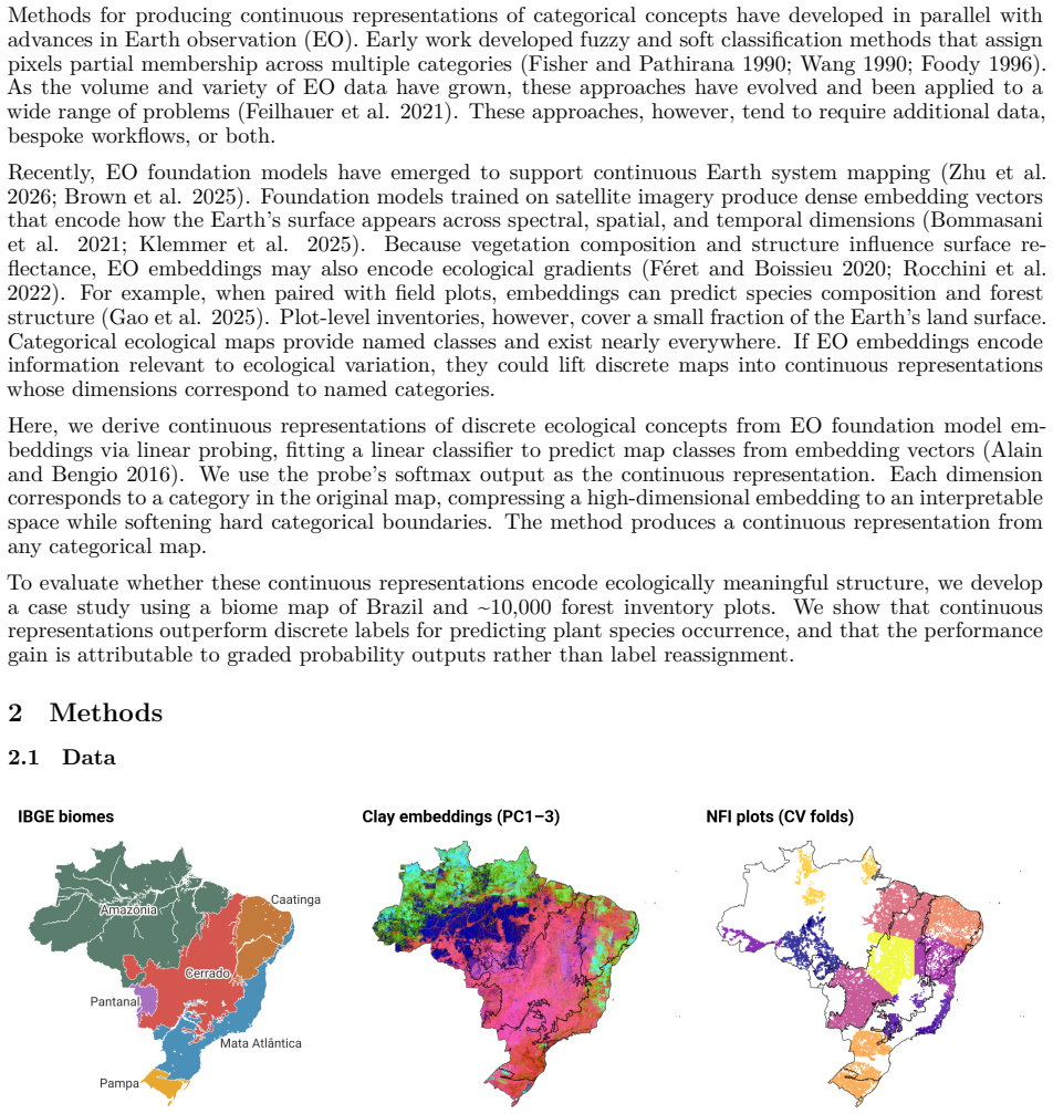
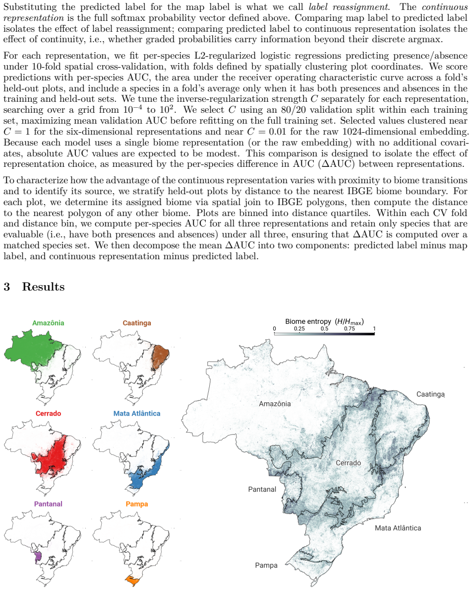
Biotic communities vary continuously across space, yet biome maps impose categorical boundaries that compress this variation, particularly at ecotones where transitional communities are ecologically distinct. Could Earth observation (EO) foundation models, which encode spectral, spatial, and temporal information with dense embeddings, convert discrete biome maps into continuous representations that better capture ecological variation? Here, we fit a linear classifier on Clay v1.5 satellite image embeddings to predict biome labels from a categorical map. The softmax output yields a continuous probability vector whose dimensions correspond to named biome classes. We evaluate this approach using six Brazilian biomes, 1.3 million embeddings, and 10,015 withheld forest inventory plots spanning 4,672 plant species. The continuous biome representation outperforms discrete biome labels for predicting species occurrence (mean per-species AUC 0.618 vs. 0.570 across 10 spatial cross-validation folds). Decomposing this gain shows that continuity in the graded probability output, rather than label reassignment, accounts for the improvement; the pattern holds across all distances from biome boundaries. The raw 1024-dimensional embedding remains the strongest predictor we tested (mean AUC 0.646 vs. 0.618), but the continuous representation recovers most of the embedding's gain over discrete labels. This simple approach provides a probabilistic replacement for categorical map labels, preserving their meaning while encoding graded variation that discrete maps suppress.
Editorial analysis
A structured set of objections, weighed in public.
Referee Report
Summary. The paper claims that training a linear classifier on Clay v1.5 Earth observation embeddings to predict categorical biome labels yields softmax probability vectors that serve as continuous biome representations; these outperform discrete biome labels when predicting occurrence of 4,672 plant species across 10,015 withheld plots (mean per-species AUC 0.618 vs. 0.570) under 10 spatial cross-validation folds, with the gain attributed to graded probabilities rather than label reassignment, and the raw 1024-d embeddings performing best (AUC 0.646).
Significance. If the central comparison holds, the method supplies an interpretable, probabilistic substitute for categorical biome maps that recovers most of the predictive value of dense EO embeddings while retaining named biome classes; this could improve modeling of transitional communities at ecotones. The use of independent species-occurrence data for evaluation and the explicit continuity-vs-reassignment decomposition are strengths.
major comments (2)
- [spatial cross-validation procedure] The spatial cross-validation procedure (abstract and results): the reported AUC comparison relies on 10 spatial folds separating the 10,015 plots, yet no details are given on fold construction (minimum inter-plot distance, clustering radius, or blocking method). Because Clay embeddings encode spatial context and species exhibit strong spatial autocorrelation, inadequate separation risks leakage that could inflate the 0.048 AUC difference; this is load-bearing for the claim that continuity drives the improvement.
- [results decomposition] Decomposition isolating continuity (results): the assertion that 'continuity in the graded probability output, rather than label reassignment, accounts for the improvement' and that the pattern holds 'across all distances from biome boundaries' requires the exact baseline construction and distance-binned analysis to be specified; without these, the attribution cannot be verified as isolating the continuity effect.
minor comments (2)
- Clarify the relationship between the 1.3 million embeddings used for classifier fitting and the 10,015 evaluation plots (abstract).
- The abstract states the continuous representation 'recovers most of the embedding's gain'; provide the exact numerical breakdown of the three AUC values in a table for direct comparison.
Simulated Author's Rebuttal
We thank the referee for their detailed and constructive report. The two major comments identify areas where the manuscript would benefit from greater methodological transparency. We address each point below and commit to revisions that strengthen the presentation without altering the core claims.
read point-by-point responses
-
Referee: The spatial cross-validation procedure (abstract and results): the reported AUC comparison relies on 10 spatial folds separating the 10,015 plots, yet no details are given on fold construction (minimum inter-plot distance, clustering radius, or blocking method). Because Clay embeddings encode spatial context and species exhibit strong spatial autocorrelation, inadequate separation risks leakage that could inflate the 0.048 AUC difference; this is load-bearing for the claim that continuity drives the improvement.
Authors: We agree that explicit details on fold construction are required to allow readers to assess the risk of spatial leakage. In the revised manuscript we will add a dedicated subsection describing the spatial blocking procedure, including the clustering algorithm, the radius used to define blocks, the minimum inter-plot distance enforced between folds, and the resulting distribution of plot-to-fold assignments. This addition will enable direct evaluation of whether the reported 0.048 AUC gain can be attributed to continuity rather than residual spatial dependence. revision: yes
-
Referee: Decomposition isolating continuity (results): the assertion that 'continuity in the graded probability output, rather than label reassignment, accounts for the improvement' and that the pattern holds 'across all distances from biome boundaries' requires the exact baseline construction and distance-binned analysis to be specified; without these, the attribution cannot be verified as isolating the continuity effect.
Authors: We accept that the current description of the continuity-versus-reassignment decomposition is insufficiently specified. In revision we will expand the relevant results section to state the precise baseline construction (i.e., how the discrete-label comparator was generated from the same embeddings), the distance metric used to compute distance from biome boundaries, the binning procedure, and the per-bin AUC differences. These additions will make the claim that graded probabilities, rather than label reassignment, drive the improvement verifiable from the reported figures and tables. revision: yes
Circularity Check
No circularity: empirical AUC comparison on independent species data
full rationale
The paper trains a linear classifier on Clay embeddings to predict categorical biome labels from a map, then uses the resulting softmax probability vector as a continuous representation. This vector is evaluated for its ability to predict species occurrence on 10,015 withheld inventory plots (4,672 species) under 10 spatial CV folds. The reported mean per-species AUC (0.618 vs. 0.570) is measured on a downstream task whose labels are independent of the biome training data; the performance metric therefore cannot reduce to the fitted biome classifier by construction. No self-definitional equations, fitted-input-as-prediction steps, or load-bearing self-citations appear in the derivation chain. The decomposition into continuity vs. reassignment is likewise an empirical contrast on the held-out species data.
Axiom & Free-Parameter Ledger
free parameters (1)
- linear classifier weights
axioms (1)
- domain assumption Clay v1.5 embeddings encode spectral, spatial, and temporal information sufficient for biome discrimination.
Reference graph
Works this paper leans on
-
[1]
Understanding intermediate layers using linear classifier probes
“Understanding Intermediate Layers Using Linear Classifier Probes. ” arXiv Preprint arXiv:1610.01644 . https://doi.org/10.48550/arXiv.1610.01644. Bommasani, Rishi, Drew A Hudson, Ehsan Adeli, Russ Altman, Simran Arber, Sydney von Arx, Michael S Bernstein, et al
work page internal anchor Pith review Pith/arXiv arXiv doi:10.48550/arxiv.1610.01644
-
[2]
On the Opportunities and Risks of Foundation Models
“On the Opportunities and Risks of Foundation Models. ” arXiv Preprint arXiv:2108.07258. https://doi.org/10.48550/arXiv.2108.07258. Brown, Christopher F, Michal R Kazmierski, Valerie J Pasquarella, William J Rucklidge, Masha Samsikova, Chenhui Zhang, Evan Shelhamer, et al
work page internal anchor Pith review Pith/arXiv arXiv doi:10.48550/arxiv.2108.07258
-
[3]
“AlphaEarth Foundations: An Embedding Field Model for Accurate and Efficient Global Mapping from Sparse Label Data. ” arXiv Preprint arXiv:2507.22291 . https://doi.org/10.48550/arXiv.2507.22291. Champreux, Antoine, Frédérik Saltré, Wolfgang Traylor, Thomas Hickler, and Corey JA Bradshaw
work page internal anchor Pith review Pith/arXiv arXiv doi:10.48550/arxiv.2507.22291
-
[4]
How to Map Biomes: Quantitative Comparison and Review of Biome-Mapping Methods
“How to Map Biomes: Quantitative Comparison and Review of Biome-Mapping Methods. ” Ecological Monographs 94 (3): e1615. https://doi.org/10.1002/ecm.1615. Chen, Theresa, and Yao-Yi Chiang
-
[5]
Mitree: Multi-Input Transformer Ecoregion Encoder for Species Distribution Modelling
“Mitree: Multi-Input Transformer Ecoregion Encoder for Species Distribution Modelling. ” In Proceedings of the 7th ACM SIGSPATIAL International Workshop on AI for Geographic Knowledge Discovery , 110–20. https://doi.org/10.1145/3687123.3698297. Curtis, John T, and Robert P McIntosh
-
[6]
An Upland Forest Continuum in the Prairie-Forest Border Region of Wisconsin
“An Upland Forest Continuum in the Prairie-Forest Border Region of Wisconsin. ” Ecology 32 (3): 476–96. https://doi.org/10.2307/1931725. Feilhauer, Hannes, András Zlinszky, Adam Kania, Giles M Foody, Daniel Doktor, Angela Lausch, and Sebastian Schmidtlein
-
[7]
“Let Your Maps Be Fuzzy!—Class Probabilities and Floristic Gradients as Alternatives to Crisp Mapping for Remote Sensing of Vegetation. ” Remote Sensing in Ecology and Conservation 7 (2): 292–305. https://doi.org/10.1002/rse2.188. Féret, Jean-Baptiste, and Florian de Boissieu
-
[8]
BiodivMapR: An R Package for 𝛼- and 𝛽-Diversity Mapping Using Remotely Sensed Images
“BiodivMapR: An R Package for 𝛼- and 𝛽-Diversity Mapping Using Remotely Sensed Images. ” Methods in Ecology and Evolution 11 (1): 64–70. https: //doi.org/10.1111/2041-210X.13310. Fisher, Peter F, and Sunil Pathirana
-
[9]
The Evaluation of Fuzzy Membership of Land Cover Classes in the Suburban Zone
“The Evaluation of Fuzzy Membership of Land Cover Classes in the Suburban Zone. ” Remote Sensing of Environment 34 (2): 121–32. https://doi.org/10.1016/0034- 4257(90)90103-S. Foody, Giles M
-
[10]
“Approaches for the Production and Evaluation of Fuzzy Land Cover Classifications from Remotely-Sensed Data. ” International Journal of Remote Sensing 17 (7): 1317–40. https://doi.or g/10.1080/01431169608948706. Freitas, Joberto V de, Yeda MM de Oliveira, Doadi A Brena, Guilherme LA Gomide, José Arimatea Silva, et al
-
[11]
The New Brazilian National Forest Inventory
“The New Brazilian National Forest Inventory. ” In In: McRoberts, Ronald E.; Reams, Gregory A.; Van Deusen, Paul C.; McWilliams, William H., eds. Proceedings of the Eighth Annual Forest Inventory and Analysis Symposium; 2006 October 16-19; Monterey, CA. Gen. Tech. Report WO-79. Washington, DC: US Department of Agriculture, Forest Service. 9-12. Gao, Xiaoj...
2006
-
[12]
“Mapping Forest Communities, Including Species Composition, Structure, and Carbon, at 10-m Resolution Using Geospa- tial Embeddings. ” SSRN Preprint . https://doi.org/10.2139/ssrn.5936862. Gleason, Henry A
-
[13]
The Individualistic Concept of the Plant Association
“The Individualistic Concept of the Plant Association. ” Bulletin of the Torrey Botanical Club 53 (1): 7–26. https://doi.org/10.2307/2479933. Hargrove, William W, and Forrest M Hoffman
-
[14]
Potential of Multivariate Quantitative Methods for Delineation and Visualization of Ecoregions
“Potential of Multivariate Quantitative Methods for Delineation and Visualization of Ecoregions. ” Environmental Management 34 (Suppl 1): S39–60. https://doi.org/10.1007/s00267-003-1084-0 . IBGE
-
[15]
Neural Hierarchical Models of Ecological Populations
“Neural Hierarchical Models of Ecological Populations. ” Ecology Letters 23 (4): 734–47. https://doi.org/10.1111/ele.13462. 7 Klemmer, Konstantin, Esther Rolf, Marc Russwurm, Gustau Camps-Valls, Mikolaj Czerkawski, Stefano Ermon, Alistair Francis, et al
-
[16]
Earth Embeddings: Towards AI-Centric Representations of Our Planet
“Earth Embeddings: Towards AI-Centric Representations of Our Planet. ” EarthArXiv Preprint. https://doi.org/10.31223/X5HX9S. Marques, Eduardo Q, Ben Hur Marimon-Junior, Beatriz S Marimon, Eraldo AT Matricardi, Henrique A Mews, and Guarino R Colli
-
[17]
Redefining the Cerrado–Amazonia Transition: Implications for Conservation
“Redefining the Cerrado–Amazonia Transition: Implications for Conservation. ” Biodiversity and Conservation 29 (5): 1501–17. https://doi.org/10.1007/s10531-019- 01720-z. Mucina, Ladislav
-
[18]
Biome: Evolution of a Crucial Ecological and Biogeographical Concept
“Biome: Evolution of a Crucial Ecological and Biogeographical Concept. ” New Phytologist 222 (1): 97–114. https://doi.org/10.1111/nph.15609. Oliveira, Gustavo Magalhães de, and Paula Sarita Bigio Schnaider
-
[19]
Implementation of the Brazilian Forest Code: A Meso-Institutional Approach
“Implementation of the Brazilian Forest Code: A Meso-Institutional Approach. ” Journal of Institutional Economics 21: e26. https: //doi.org/10.1017/S1744137425100143. Olson, David M, Eric Dinerstein, Eric D Wikramanayake, Neil D Burgess, George VN Powell, Emma C Underwood, Jennifer A D’amico, et al
-
[20]
“Terrestrial Ecoregions of the World: A New Map of Life on Earth: A New Global Map of Terrestrial Ecoregions Provides an Innovative Tool for Conserving Biodiversity. ” BioScience 51 (11): 933–38. https://doi.org/10.1641/0006-3568(2001)051%5B0933: TEOTWA%5D2.0.CO;2. Omernik, James M, and Glenn E Griffith
-
[21]
Clustering Biomes from Space: From Pixels to Foundation Models
“Clustering Biomes from Space: From Pixels to Foundation Models. ” SSRN Preprint. https://doi.org/10.2139/ssrn.6876998. Risser, Paul G
-
[22]
The Status of the Science Examining Ecotones
“The Status of the Science Examining Ecotones. ” BioScience 45 (5): 318–25. https: //doi.org/10.2307/1312492. Rocchini, Duccio, Maria J. Santos, Susan L. Ustin, Jean-Baptiste Féret, Gregory P. Asner, Carl Beierkuhn- lein, Michele Dalponte, et al
-
[23]
The Spectral Species Concept in Living Color
“The Spectral Species Concept in Living Color. ” Journal of Geo- physical Research: Biogeosciences 127 (9): e2022JG007026. https://doi.org/10.1029/2022JG007026. Smith, Jeffrey R, Andrew D Letten, Po-Ju Ke, Christopher B Anderson, J Nicholas Hendershot, Manpreet K Dhami, Glade A Dlott, et al
-
[24]
“A Global Test of Ecoregions. ” Nature Ecology & Evolution 2 (12): 1889–96. https://doi.org/10.1038/s41559-018-0709-x . Tansley, Arthur G
-
[25]
The Use and Abuse of Vegetational Concepts and Terms
“The Use and Abuse of Vegetational Concepts and Terms. ” Ecology 16 (3): 284–307. https://doi.org/10.2307/1930070. Wang, Fangju
-
[26]
Fuzzy Supervised Classification of Remote Sensing Images
“Fuzzy Supervised Classification of Remote Sensing Images. ” IEEE Transactions on Geoscience and Remote Sensing 28 (2): 194–201. https://doi.org/10.1109/36.46698. Whittaker, Robert H
-
[27]
Vegetation of the Great Smoky Mountains
“Vegetation of the Great Smoky Mountains. ” Ecological Monographs 26 (1): 1–80. https://doi.org/10.2307/1943577. Wilcox, Allen R
-
[28]
Indices of Qualitative Variation and Political Measurement
“Indices of Qualitative Variation and Political Measurement. ” Western Political Quarterly 26 (2): 325–43. https://doi.org/10.1177/106591297302600209. Zhu, Xiao Xiang, Zhitong Xiong, Yi Wang, Adam J. Stewart, Konrad Heidler, Yuanyuan Wang, Zhenghang Yuan, Thomas Dujardin, Qingsong Xu, and Yilei Shi
-
[29]
https://doi.org/10.1038/s43247-025-03127- x. 8
discussion (0)
Sign in with ORCID, Apple, or X to comment. Anyone can read and Pith papers without signing in.